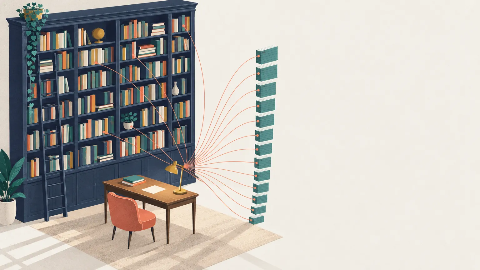
In February 2023 Meta released LLaMA, a family of four language models from 6.7 to 65.2 billion parameters. The smallest one fits on a single GPU: its 6.74 billion parameters take 13.5 GB at two bytes each (FP16, computed). Serve it to 32 users at once, each with a full 2,048-token context, and the GPU must also hold 32 GiB of keys and values that the model computed for those users’ earlier tokens (computed below). That is more than twice the memory of the model itself, and each step that produces the next token for all 32 users reads all of it.
LLaMA 1 is a convenient starting point for this series. It collected the design choices that had settled by early 2023 (pre-normalization with RMSNorm, the SwiGLU feed-forward unit, rotary position embeddings, no biases) into one plain, well-documented decoder, and many open models since have started from that recipe. Every model in the map keeps its skeleton: an embedding, a stack of residual layers, an output head. Most of what changed is a response to cost. The largest models in the map have 1.6 trillion (DeepSeek-V4-Pro) and 2.8 trillion (Kimi K3) total parameters, 25 and 43 times LLaMA-65B; they accept contexts of 128K to 1M tokens instead of 2,048; and they are served to many users at once. This article describes the 2023 baseline, then builds the cost model that the rest of the series uses to explain why each part was changed.
The early modern decoder: LLaMA 1
From text to vectors and back
A language model reads text as a sequence of tokens, pieces of words drawn from a fixed
vocabulary. LLaMA’s tokenizer is byte-pair encoding with 32,000 entries (vocab_size: 32000
in the released config), which splits “all numbers into individual digits” and falls back to
raw bytes for characters it has never seen (Touvron et al., 2023, §2.1).
The model turns each token id into a vector of width by looking up a row of an embedding
table , with the vocabulary size. For LLaMA-7B,
. These vectors then pass through identical decoder layers ( for 7B).
At the top, a final normalization and an output matrix
turn each position’s vector into scores, the logits, and a softmax over them gives the
probability of every possible next token. LLaMA keeps the two tables separate
(tie_word_embeddings: false).
The model is trained to predict token from tokens , at every position of a training sequence at once. To generate, you run it, pick a next token from the distribution at the last position, append that token to the input, and run again. Generating one token at a time, each conditioned on all the earlier ones, is called autoregressive decoding.
The residual stream
Each decoder layer reads a matrix (one row per token, tokens) and adds something to it. Each of its two sub-layers computes an update from a normalized copy of and adds the update back:
def layer(x, p):                      # x: [T, d]
    x = x + attention(rmsnorm(x, p.attn_norm), p)
    x = x + swiglu_ffn(rmsnorm(x, p.ffn_norm), p)
    return x
The running sum is called the residual stream. It is the only path by which information travels from one layer to the next. Because each layer adds to it, the Jacobian of one layer’s output with respect to its input is , where is the Jacobian of the sub-layer branch, so the gradient reaching the lowest layers always contains an identity term (the argument of the pre-activation ResNet, He et al., 2016).
The original Transformer normalized each sub-layer’s output, after the addition (post-normalization). LLaMA normalizes the input of each sub-layer instead (pre-normalization), “to improve the training stability” (§2.2), as GPT-3 did. With post-normalization the identity path passes through a normalization in every layer, and such models need a careful learning-rate warm-up to train (Xiong et al., 2020). Pre-normalization keeps the path clean, at a price: nothing rescales the stream itself, and its magnitude tends to grow with depth, a problem that R1 and R2 return to.
The normalization is RMSNorm (Zhang and Sennrich, 2019), which rescales each row to unit root-mean-square and multiplies by a learned per-channel gain . Unlike LayerNorm it neither subtracts the mean nor adds a bias:
def rmsnorm(x, w, eps=1e-6):          # x: [T, d], w: [d]
    return x * rsqrt(mean(x**2, dim=-1, keepdim=True) + eps) * w
Attention moves information between positions: row of its output depends on rows of its input. We call it the token mixer. The feed-forward network works on each row separately, mixing the channels of one token. We call it the channel mixer. The map uses the same two words, because later models replace each one independently.
The token mixer: causal multi-head attention
LLaMA’s multi-head attention has heads of dimension , with (32 heads of 128
dimensions for 7B). Each head projects the input into queries, keys and values, compares each
query with the keys of the same and earlier positions, and returns a weighted sum of the
corresponding values. In einsum notation, with the projection weights stored per head (index
letters: t, s positions, h heads, c channels within a head, d model width):
def attention(x, p):                  # x: [T, d]
    pos = arange(T)
    q = rope(einsum("td,dhc->thc", x, p.Wq), pos)   # Wq, Wk, Wv: [d, h, d_h]
    k = rope(einsum("td,dhc->thc", x, p.Wk), pos)
    v =      einsum("td,dhc->thc", x, p.Wv)
    s = einsum("thc,shc->hts", q, k) / sqrt(d_h)    # scores: [h, T, T]
    s = where(pos[None, :, None] >= pos[None, None, :], s, -inf)   # causal: s <= t only
    a = softmax(s, dim=-1)
    o = einsum("hts,shc->thc", a, v)                # [T, h, d_h]
    return einsum("thc,hcd->td", o, p.Wo)           # Wo: [h, d_h, d]
The causal mask makes the model autoregressive: position may attend only to positions , so its output never depends on tokens it is supposed to predict.
A single attention read has no notion of order: permuting the earlier tokens only permutes the terms of the weighted sum, so the output is unchanged. (A stack of causal layers can still infer position, because the mask lets each position see a different number of tokens; Haviv et al., 2022, trained decoders without any position encoding. T4 returns to such NoPE layers.) LLaMA supplies position with rotary position embeddings (RoPE; Su et al., 2021), applied “at each layer of the network” in place of absolute position vectors added to the input (§2.2). RoPE splits each query and key into pairs of coordinates and rotates pair of the vector at position by the angle , with frequencies . Rotations compose, so the dot product depends on the offset and not on and separately. RoPE has no parameters. T4 covers how models stretch these frequencies to longer contexts.
Written as above, attention builds the full score matrix. LLaMA’s training code avoided that with a fused kernel from the xformers library that, in the paper’s words, works “by not storing the attention weights and not computing the key/query scores that are masked” (§2.4); FlashAttention (Dao et al., 2022) is the standard form of that idea. The result is the same; the kernel moves far fewer bytes, and skipping the masked half of the scores halves their FLOPs, which the counts below already assume.
The channel mixer: the SwiGLU feed-forward unit
The original Transformer used a two-matrix feed-forward network with a ReLU and a hidden width of . LLaMA uses SwiGLU (Shazeer, 2020), a member of the gated linear unit family of Dauphin et al. (2017), whose multiplicative gating goes back to the LSTM. It has two input projections: one passes through the SiLU function and scales the other elementwise, then an output projection maps back to width .
def swiglu_ffn(x, p):                 # W1, W3: [d, d_ff]; W2: [d_ff, d]
    return (silu(x @ p.W1) * (x @ p.W3)) @ p.W2
Three matrices instead of two would cost 50% more parameters at the same hidden width, so LLaMA
shrinks the width to (§2.2), rounded up to a multiple of 256 in the
reference code. For 7B that is (intermediate_size: 11008), and
: the same parameters and FLOPs as a ReLU network of
width . Shazeer reports better quality at that matched budget. C1 covers the gated
family.
The whole model
def model(tokens):                    # tokens: [T] ints
    x = W_emb[tokens]                 # [T, d], a row lookup
    for p in layers:
        x = layer(x, p)
    return rmsnorm(x, final_norm) @ W_out   # logits: [T, V]
That is all of LLaMA 1 at inference time. No layer has a bias, there is no dropout, and every layer has the same shape.
Total: 2 × 131.1M (tables) + 32 × (67.1M attention + 135.3M feed-forward + 8,192 norm weights) + 4,096 = 6.738B parameters.Grey tags: articles that change the part (T token mixer, C channel mixer, R norms and residual, M embedding, P output, X input).
Where the parameters are
Counting the matrices gives the size. Per layer, attention has four matrices () and the feed-forward unit three matrices (). With the embedding and output tables (), LLaMA-7B has 6.738 billion parameters (computed; the paper rounds to 6.7B). Nearly two thirds of them, 64%, are in the feed-forward units, 32% in attention, and 3.9% in the two vocabulary tables. With a layer has about parameters, so the tables’ share relative to the layers is about : 4.1% for 7B and 0.8% for 65B, which is both wider and deeper.
embedding + outputattentionfeed-forwardshare of parameters, linear 0 to 100%; total at right
Training cost follows from the parameter count. A matrix multiplication costs two floating-point operations (FLOPs: a multiply and an add) per weight per token in the forward pass, and about four in the backward pass (two for the gradient with respect to the input, two for the gradient with respect to the weight). Training therefore costs about FLOPs for parameters and tokens (Kaplan et al., 2020), plus attention, which this count leaves out. LLaMA-65B saw 1.4 trillion tokens, about FLOPs (computed). The paper reports about 380 tokens per second per GPU on 2,048 A100s, for about 21 days. That rate is TFLOP/s per GPU, 48% of an A100’s 312 TFLOP/s BF16 peak (computed). This ratio of useful model FLOPs to peak is called model FLOP utilization. The GPU actually did somewhat more arithmetic than this, because the paper recomputes some activations in the backward pass (§2.4). Training uses about half of the GPU’s arithmetic; decode, as the next sections show, uses a few percent at most.
Generating text: prefill, decode and the KV cache
Run the model on a prompt of 1,000 tokens and it computes all 1,000 rows in parallel, with large matrix multiplications. That phase is called prefill. Its last row gives the first new token. Now the model must produce token 1,002, then 1,003, and so on, one forward pass per token. This phase is called decode.
The naive way to decode reruns the model on the whole sequence each time. That repeats almost all the work: because of the causal mask, rows of every layer are exactly what they were in the previous pass. The only thing the new token needs from them is, in each layer and head, their keys and values. So inference engines compute the keys and values once and keep them. The store is the KV cache. A decode step then runs the model on one row: it computes that token’s query, key and value in every layer, appends the key and value to the cache, and attends from its query over everything cached. The result is the same as recomputing everything, up to rounding.
def attention_step(x, p, cache, t):   # x: [1, d], the token at position t
    q = rope(einsum("td,dhc->thc", x, p.Wq), [t])
    cache.k = concat([cache.k, rope(einsum("td,dhc->thc", x, p.Wk), [t])])   # [t+1, h, d_h]
    cache.v = concat([cache.v,      einsum("td,dhc->thc", x, p.Wv)])
    s = einsum("thc,shc->hts", q, cache.k) / sqrt(d_h)   # [h, 1, t+1]: no mask needed
    o = einsum("hts,shc->thc", softmax(s, dim=-1), cache.v)
    return einsum("thc,hcd->td", o, p.Wo)
LLaMA’s reference code does exactly this, with the cache preallocated as one tensor per layer of shape (sequences, maximum length, heads, head dimension).
keyvaluehatched: already cachedsolid: computed in this stepthe new query reads
prefill: 6 tokens, all computed together
cache: 6 tokens × 32 layers × 16 KiB = 3 MiB
The cache is large. Per token and layer it holds one key and one value vector for each key/value head. Call the number of key/value heads : in LLaMA every query head has its own, so , but later designs let several query heads share one, down to a single shared head (, multi-query attention; T1). With bytes per stored number,
For LLaMA, . For 7B in FP16 () this is KiB per
layer, 512 KiB per token over 32 layers, and 1 GiB for one 2,048-token sequence (computed; 1 GiB =
bytes, 7% more than a decimal GB, the unit GPU memory is sold in). For 65B it is 2.5 MiB per
token and 5 GiB per sequence. The 32 GiB of the opening is 32 sequences of 2,048 tokens, which are
also the default sizes in the reference code’s ModelArgs (max_batch_size: 32,
max_seq_len: 2048).
The cache grows linearly with context length and with the number of sequences served together. And it belongs to its sequence: two requests share cache entries only for an identical prefix, such as a common system prompt. Both facts matter for everything below.
A cost model in three numbers
To see what limits each phase, you need three properties of the accelerator. An NVIDIA H100 (SXM) can do about 989 TFLOP/s of dense BF16 arithmetic, read 3.35 TB/s from its main memory (HBM, the GPU’s high-bandwidth DRAM), and hold 80 GB in it. (FP16 and BF16 are both two-byte number formats; they differ in how the bits are split between range and precision, not in size.) The first two numbers set the speed limits. Their ratio,
is the arithmetic intensity, in FLOPs per byte read from memory, that a computation needs to keep the arithmetic units busy. (T1 rounds the same figures to 990 and “about 300”.) A computation that does fewer FLOPs per byte waits for memory, and its time is bytes divided by bandwidth: it is memory-bound. One that does more is compute-bound, and its time is FLOPs divided by peak. This two-regime picture is the roofline model (Williams et al., 2009). It ignores kernel launch overheads, on-chip caches and communication between GPUs, so it gives lower bounds on time. It still identifies which resource limits each phase, and the arguments in this series rely only on that.
decode, LLaMA-7B at 2,048 tokensprefilldashed: the most any batch reaches
Prefill is compute-bound
A prefill of tokens multiplies every weight matrix by rows at once. Each weight is read from memory once and used times, so the matrix multiplications do about FLOPs per byte (two FLOPs per weight per token, two bytes per weight). Attention adds FLOPs: every token attends on average to half the prompt, and each of those pairs costs FLOPs per layer. For LLaMA-7B and a 2,048-token prompt,
against 13.5 GB of weights read once, about 2,100 FLOPs per byte, far right of the ridge (computed). At peak the prefill would take 29 ms. Its time sets the time to first token, the wait before an answer starts appearing.
Decode is memory-bound
A decode step for one sequence runs the same matrices on a single row. It still reads all 13.5 GB of weights, and does 13.5 GFLOP with them: one FLOP per byte. Attention is no better. For each head and each cached token, the step reads a key and a value, numbers or bytes, and does one dot product and one scaled addition, FLOPs. That is again one FLOP per byte. At 2,048 tokens of context the step reads 14.6 GB (weights plus 1 GiB of cache) in 4.3 ms; the arithmetic would take 15 µs. The model can produce at most about 230 tokens per second for that one user, and the GPU’s arithmetic units are idle more than 99% of the time (computed).
Batching is the standard remedy. If sequences decode together, each weight read serves all of them, and the intensity of the weight multiplications rises to about . Weights alone would make decode compute-bound at a batch near 295. But each sequence reads its own cache, so a larger batch adds cache bytes exactly as fast as it adds attention work. A decode step reads
for sequences at context length (all equal, for simplicity; real servers mix lengths, and the cache term is then a sum over sequences). For LLaMA the two terms have a simple ratio. With and , the cache of one sequence equals the weights at
for 7B (computed). Writing , the bytes are and the FLOPs , so the intensity of a whole decode step is
At batch 1 it is exactly 1 for any context length. As grows, it approaches the bound on the right, which is reached when the cache dominates. At the bound is 13.6 FLOPs per byte, and no batch size, however large, gets decode within a factor of 20 of the ridge at 295 (computed). To reach 295 the context would have to be shorter than 87 tokens.
Memory capacity stops the batch earlier still. On an 80 GB H100, weights plus cache leave room for 61 sequences of 2,048 tokens (ignoring activations and allocator overhead). At that batch a step reads 79 GB, 83% of it cache, runs at 11.2 FLOPs per byte, 4% of what the arithmetic units could do, and produces about 2,600 tokens per second in total, 42 per sequence (all computed, at vendor peak bandwidth for LLaMA-7B).
weights, read once per stepKV cache, one per sequence (hatched: cached)bytes per decode step, linear axis from 0 · context T is log scale
fits in one H100 (80 GB); at T = 2K, at most 61 sequences fit.
- read per step
- 14.55 GB, 7.4% cache
- step time
- 4.34 ms, memory-bound
- tokens/s in total
- 230
- tokens/s per sequence
- 230
- FLOPs per byte
- 1.0 (ridge ≈ 295)
- share of peak FLOP/s
- 0.34%
Roofline lower bounds at vendor peak (989 TFLOP/s, 3.35 TB/s per H100); two GPUs add up, communication ignored.
Decode speed is set by bytes, so a design that reads fewer bytes per token is faster even if it does more arithmetic per byte. For LLaMA-7B at 2,048 tokens, between 26 times (batch 61) and 295 times (batch 1) more arithmetic would fit in the same time. And since the cache sets how many sequences fit, a smaller cache per token means larger batches and more tokens per second per GPU, the number that sets the price of serving.
Three levers outside the layer design act on the same byte count. Storing numbers in fewer bits
shrinks : many models in the map ship their weights in FP8 (DeepSeek-V3.2, GLM-5.3, the MiMo
models; quant_method: fp8 in their configs), gpt-oss and Kimi K3 store their routed experts in the
4-bit MXFP4 format, and servers often store the cache in FP8. Decoding several tokens per step raises intensity directly:
in speculative decoding a small, cheap draft proposes a few tokens and the large model checks them
all in one forward pass, reading its weights and cache once for several tokens. Some models train
extra heads for this (multi-token prediction, P1). And sequences that share a prefix
can share its cache. This series is about the layer design, but its byte counts are always
compared at one stated , BF16 unless said otherwise.
Long contexts: where attention takes over
At 2,048 tokens, attention is a small part of LLaMA’s cost. Count FLOPs per token per layer. The projections (four attention matrices and three feed-forward matrices) cost , 405 MFLOP for 7B, whatever the context. A decoded token attends to earlier tokens at FLOPs each; a prefill token attends to of them on average. So in prefill, attention matches the projections at
for LLaMA-7B (computed), and its share of prefill FLOPs is 4% at 2,048 tokens, 73% at 128K and 96% at 1M. Decode is limited by bytes, and there the cache term crosses the weights twice as early, at : for a single sequence, the cache is 7% of the bytes read per step at 2,048 tokens, 84% at 128K and 98% at 1M (computed). At 1M tokens, LLaMA-7B’s shape would need 512 GiB of cache for that one sequence.
Long context therefore raises both phases’ costs through the term that grows with . The series covers three kinds of answer. T1 stores fewer numbers per token (grouped-query and latent attention). T2 stores a bounded amount per layer (sliding windows, and recurrent layers that keep a fixed-size state), and T3 keeps every token but reads only a selected subset. T5 keeps full attention in only a few layers, or shares one cache across layers.
Mixture of experts: moving the weight bytes
The other byte term is the weights, and the largest share of them is in the feed-forward units. A mixture-of-experts (MoE) layer, an idea that goes back to Jacobs et al. (1991) and was scaled to language models with a sparse top- gate by Shazeer et al. (2017), replaces the one feed-forward unit with feed-forward units, the experts, each usually much narrower than a dense layer’s, and a router that sends each token to of them. The router is a small linear layer that scores every expert. The top- choice itself passes no gradient; the router learns through the scores of the experts it picked, which weight their outputs. Left alone, that tends to collapse onto a few experts, which is why MoE models usually add a balancing loss or bias (C3).
A token’s FLOPs are set by the parameters it uses, the active parameters. The memory needed is set
by all of them, the total. Qwen3.5-397B-A17B, for example, has 512 routed experts per layer and
routes each token to 10 (num_experts: 512, num_experts_per_tok: 10), plus one shared expert that
every token uses; its name gives 397B total and 17B active parameters. In BF16 its weights fill
794 GB, ten 80 GB GPUs, while a single token touches 34 GB of them (computed).
Prefill and training pay FLOPs for 17B parameters while the model stores 397B. A decode step at batch 1 reads only the experts its token uses. With more sequences in the batch, tokens are routed to different experts and the step must read the union. If each token chose of experts uniformly and independently, a batch of tokens would touch on average
experts per layer: 367 of 512 at , almost all at (computed; real routing is neither uniform nor independent). Once most experts are read, each expert’s weights serve only the about tokens routed to it, so the expert matrices run at about FLOPs per byte: about 5 at batch 256. Reaching the ridge of 295 would take about 15,000 tokens per step (computed). The same holds in prefill: a 2,048-token prompt sends about 40 tokens to each expert, so those multiplications run near 40 FLOPs per byte, memory-bound even in the phase that is otherwise compute-bound.
This is why MoE models are served across many GPUs with each GPU holding a subset of the experts (expert parallelism): requests from many GPUs pool their tokens, so each expert sees a large batch. The pooling has a communication cost. Each token’s vector of width has to be sent to the GPUs holding its experts and the results sent back, an exchange called all-to-all, whose volume grows with per token per layer. C2 covers the design space.
Prefill comes back
The cost model so far treats a request as one prompt followed by a long answer. In agentic work, a request is many short turns over one long context: a coding agent calls a tool, receives a few thousand tokens of output, appends them to a context of perhaps 100K tokens, and asks the model to continue, many times per task. Inference engines keep the cache of earlier turns so that only new tokens need prefill, a technique called prefix caching. When that cache was evicted (dropped to free memory for other requests), the whole context is prefilled again. The DeepSeek-V4.1-Flash report states the problem directly: “In agentic workflows, frequent tool calls generate extensive prefill requests, imposing severe computational overhead when KV caches miss” (§2.2). Even on a cache hit, each new token attends over the whole cached context. In LLaMA-7B’s shape, attending over 100K tokens costs about four times the FLOPs of the token’s projections (computed), so that prefill is mostly attention.
Re-prefilling a long context is compute-bound, so designs aimed at it cut FLOPs per prompt token. DeepSeek-V4.1-Flash splits its stack into a lower half (the “encoder”) and an upper half. Most of its layers attend both to a recent window of tokens and to entries selected from a compressed cache of the whole context, which the report calls global attention. In the upper half, the global keys and values are projected from the encoder’s final output instead of being computed layer by layer, so a prompt token’s global cache is complete after the lower half. The upper half’s window caches still need the upper layers; the report runs only the last window of the prompt through them (“SWA Bounded Replay”), an approximation it says barely affects quality. Generated tokens run through all layers. The report gives 8B activated parameters per token in prefill against 16B in decode, and says this “reduces nearly half of the prefill computation while maintaining performance comparable to the baseline”. T5 covers this design (the report calls it a causal encoder-decoder, CED) and its predecessor YOCO.
What the architecture does to the serving system
Some costs don’t appear in FLOP or byte counts and show up only when the model is served.
Large models don’t fit on one GPU. The usual way to split a layer is tensor parallelism: each GPU holds a slice of every weight matrix, and for attention the natural slice is a set of heads, with those heads’ cache on the same GPU. A design with few key/value heads has little to split; with one shared head, every GPU must hold a full copy of the cache, and serving stacks often switch to running attention data-parallel instead (each GPU serves different requests with its own cache).
Real servers don’t decode a fixed batch in lock-step. They use continuous batching, adding and removing requests at every step, and mix chunks of new prompts into decode steps so the GPU’s spare arithmetic during decode is used for prefill. The byte and FLOP counts above still apply per step; they are summed over whatever the step contains.
A cache that is not a simple per-token, per-layer array complicates memory management. Serving engines allocate the cache in fixed-size blocks of tokens (PagedAttention; Kwon et al., 2023), which works neatly when every layer stores the same thing per token. Models that mix sliding-window layers, recurrent layers and compressed caches have several kinds of state with different sizes and lifetimes, and a prefix cache must be able to resume from a saved point in each of them. A recurrent state, for example, can only be resumed at positions where a snapshot was saved. The model reports in the map spend pages on these kernels and cache layouts, because a design that the serving stack cannot run efficiently does not deliver its paper savings.
The cost terms and the articles that change them
| Cost term | What sets it | Phase it limits | Articles |
|---|---|---|---|
| KV bytes per token per layer | decode bytes, batch size | T1 | |
| Tokens kept or read per layer | , or a window, a fixed state, a selection | decode bytes, prefill FLOPs | T2, T3 |
| Layers with a growing cache | , or the number of global layers | decode bytes, prefill FLOPs | T5 |
| Weight bytes and FLOPs per token | active parameters | decode bytes at small batch, prefill, training | C2 |
| Capacity outside the FLOP budget | parameters looked up, not multiplied | memory | M1 |
| Tokens per forward pass | one, or several checked at once | decode steps | P1 |
| Training stability at scale | norm placement, growth of attention logits and of the residual stream | training | R1, R2 |
Position encoding (T4), sinks and output gates (T6) and multimodal input (X1) mostly affect quality; each of those articles also names its cost.
Where the models in the map sit
The table puts LLaMA 1 next to a selection of models in the map. Shapes, expert counts and layer
types are from each model’s config.json. Total and active parameters are from the model’s report or
model card, or, for Qwen3.5, its name; a dash means no first-party source in the corpus states them.
KV bytes are per token for one layer whose cache grows with context, in BF16, computed as
(for latent attention, MLA, the 512-number latent plus a 64-number position key, times
).
| Model | Layers | Context | FFN | Token mixers | KV per global layer | Total / active | |
|---|---|---|---|---|---|---|---|
| LLaMA-7B (2023) | 32 | 4,096 | 2K | dense, 11,008 | 32 MHA | 16 KiB | 6.7B / 6.7B |
| LLaMA-65B (2023) | 80 | 8,192 | 2K | dense, 22,016 | 80 MHA | 32 KiB | 65.2B / 65.2B |
| Gemma 4 31B | 60 | 5,376 | 256K | dense, 21,504 | 10 global (K=V), 50 SWA | 4 KiB | 31B dense |
| gpt-oss-120b | 36 | 2,880 | 128K | 128 experts, top 4 | 18 GQA, 18 SWA | 2 KiB | 116.8B / 5.1B |
| Qwen3.5-397B-A17B | 60 | 4,096 | 256K | 512 experts, top 10, 1 shared | 15 GQA, 45 linear | 2 KiB | 397B / 17B |
| MiniMax-M3 | 60 | 6,144 | 1M | 128 experts, top 4, 1 shared | 60 GQA, 57 of them with block selection | 2 KiB | ~428B / ~23B |
| Laguna-S-2.1 | 48 | 3,072 | 1M | 256 experts, top 10, 1 shared | 12 GQA, 36 SWA | 4 KiB | 118B / 8B |
| DeepSeek-V3.2 | 61 | 7,168 | 160K | 256 experts, top 8, 1 shared | 61 MLA with token selection | 1,152 B + index keys | – |
| DeepSeek-V4-Pro | 61 | 7,168 | 1M | 384 experts, top 6, 1 shared | compressed + SWA | see T3 | 1.6T / 49B |
| Kimi K3 | 93 | 7,168 | 1M | 896 experts, top 16, 2 shared | 24 MLA, 69 KDA | 1,152 B | 2.8T / 104B |
| Nemotron 3 Ultra | 108 blocks | 8,192 | 256K | 512 experts, top 22, 1 shared | 12 GQA, 48 Mamba | 1 KiB | 550B / 55B |
How to read the token-mixer column. MHA is LLaMA’s multi-head attention. GQA (grouped-query attention) and MLA (multi-head latent attention) are full attention with a smaller cache per token (T1); K=V stores one vector per head that serves as both key and value. A “global” layer attends to the whole context. SWA (sliding-window attention) attends only to the most recent tokens, and “linear” (Gated DeltaNet), KDA (Kimi Delta Attention) and Mamba layers keep a recurrent state of fixed size (T2); their memory does not grow with context and is not in the KV column. Block and token selection read only part of a full cache, and need a small extra index cache (T3); DeepSeek-V4 compresses the cache along the sequence (T3). A shared expert is one that every token uses in addition to its routed ones (C2).
Other notes. Contexts are max_position_embeddings in units of 1,024 tokens (K) or (1M).
Nemotron 3 Ultra’s 108 blocks are 48 Mamba, 48 MoE and 12 attention blocks, each a single sub-layer.
Gemma 4’s sliding-window layers store more per token than its global ones (16 key/value heads of 256,
16 KiB), but only for the last 1,024 tokens. MiniMax-M3’s parameter counts are from its model card,
Laguna’s from Poolside’s release post, and Kimi K3’s from its technical report.
Easy to get wrong
- A decode step’s time follows the bytes it reads. Two models with the same FLOPs per token can differ several-fold in decode speed, and an MoE model’s speed depends on its batch.
- Batching amortizes only the weight reads. Each sequence still reads its whole cache, so attention costs the same bytes per token at any batch size.
- “Memory-bound” doesn’t mean the GPU is out of memory. It means the time is set by memory bandwidth. Memory capacity is a separate limit, and the KV cache drives both.
- Prefill and decode are limited by different things, so a design can help one and hurt the other. A claim of “faster inference” needs its phase, batch size and context length.
- Decoding with a KV cache gives the same result as recomputing every earlier token, up to rounding. What it costs is memory.
- The roofline numbers here are lower bounds at vendor peaks. Use them to tell which resource limits a phase; measured step times will be longer, and multi-GPU serving adds communication.
Check yourself
- LLaMA-13B has 40 layers and , with multi-head attention. How large is the KV cache in
FP16 for 16 sequences of 2,048 tokens?
Answer
Per token per layer KiB; × 40 layers = 800 KiB per token; × 2,048 tokens × 16 sequences = 25 GiB. - On one H100, what is the fastest LLaMA-13B could decode at batch 1, ignoring the cache?
Answer
The weights are about 26 GB (13.0B × 2 bytes). Reading them at 3.35 TB/s takes about 7.8 ms per token, so at most about 130 tokens per second. - Why does a larger batch raise the arithmetic intensity of the weight multiplications but not of
attention?
Answer
The weights are shared by all sequences in the batch, so one read serves tokens. Each sequence’s keys and values belong only to it, so a larger batch adds bytes and FLOPs in proportion. - A variant of LLaMA-7B uses multi-query attention: one key/value head per layer () instead of
32, with everything else unchanged (ignore the small change in the weights). Which phase gets
faster, and roughly by how much, at batch 61 and 2,048 tokens?
Answer
Decode. The cache bytes fall 32-fold, from about 65 GB to 2 GB per step, so a step reads about 15.5 GB instead of 79 GB and is about five times faster. Prefill, which is compute-bound, barely changes.
In the map
Methods
- RMSNorm 2 sources
- Pre-LN 1 source
- SwiGLU 2 sources
- Rotary Position Embedding 6 sources
- FlashAttention 2 sources
- Mixture of experts 113 sources
- Expert parallelism 12 sources
- Speculative decoding 15 sources
- Prefix caching 10 sources
- Continuous batching 1 source
Taxonomy nodes
- model architecture 19 methods
Further reading
- Touvron et al., LLaMA: Open and Efficient Foundation Language Models (2023), arXiv:2302.13971. §2 has the architecture and training recipe in two pages.
- Pope et al., Efficiently Scaling Transformer Inference (2022), arXiv:2211.05102. The prefill and decode cost analysis, including how partitioning across chips changes it.
- Kwon et al., Efficient Memory Management for Large Language Model Serving with PagedAttention (2023), arXiv:2309.06180. How the KV cache is allocated in practice, and how much memory naive allocation wastes.
- Williams, Waterman and Patterson, Roofline (2009), Communications of the ACM 52(4). The two-regime performance model.
- Kaplan et al., Scaling Laws for Neural Language Models (2020), arXiv:2001.08361. The training estimate and the per-token FLOP count.
- Dao et al., FlashAttention (2022), arXiv:2205.14135. Exact attention without materializing the score matrix.
- Xiong et al., On Layer Normalization in the Transformer Architecture (2020), arXiv:2002.04745. Why post-normalization needs warm-up and pre-normalization does not.
- Shazeer, GLU Variants Improve Transformer (2020), arXiv:2002.05202. SwiGLU and its matched-budget comparison.
- Zhang and Sennrich, Root Mean Square Layer Normalization (2019), arXiv:1910.07467. RMSNorm.
- Su et al., RoFormer (2021), arXiv:2104.09864. Rotary position embeddings.
- Haviv et al., Transformer Language Models without Positional Encodings Still Learn Positional Information (2022), arXiv:2203.16634.
- Shazeer et al., Outrageously Large Neural Networks: The Sparsely-Gated Mixture-of-Experts Layer (2017), arXiv:1701.06538. Top- routing and the balancing loss.
- DeepSeek-V4.1-Flash technical report (2026), §2.2. Prefill cost in agentic workloads and the causal encoder-decoder.