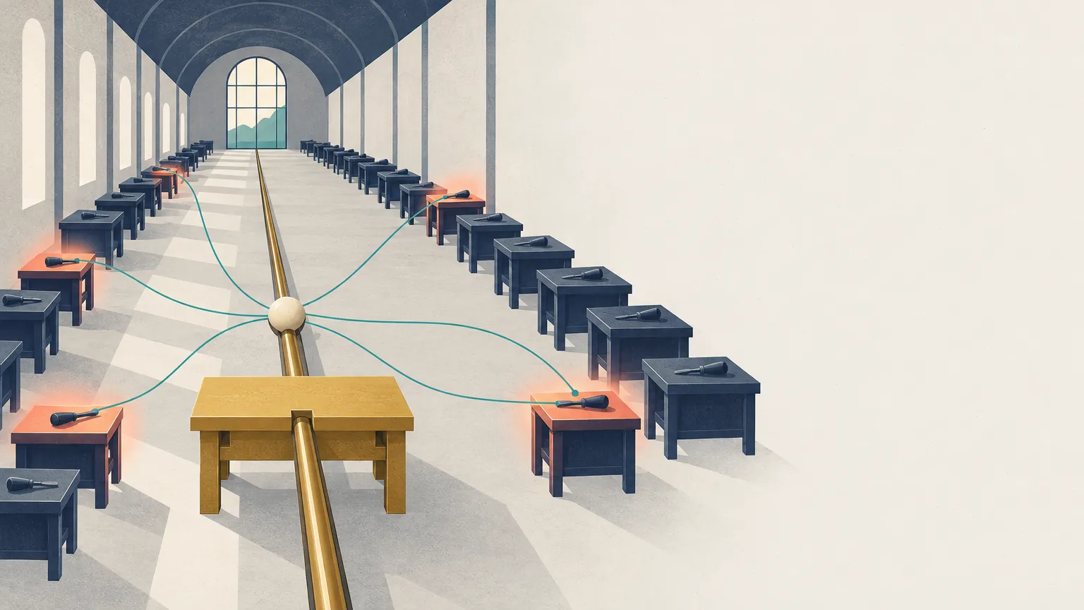
A Kimi K3 layer holds 896 experts and uses 16 of them for each token. Across the model that comes to
2.78 trillion parameters, of which a token activates 104 billion (K3 report, Table 1). In BF16, two
bytes per number, the model would fill 5.6 TB. K3 ships its routed experts in a 4-bit format
(mxfp4-pack-quantized), which brings that to about 1.5 TB (computed, ignoring scales), still far more
than one GPU holds.
Labs build models this way because quality rises with total parameters, with diminishing returns, while compute follows active parameters. Expert counts stop short of a million because the other costs follow other things. Storage follows the total. Weight reads follow the active set at small batch and the total at large batch. Traffic between GPUs follows the number of active experts times the width of the vector sent to each.
Thirty-three of the 35 models tracked on this site use such a layer, from 14 labs, with different answers on how many experts, how wide, how many active, which always run, and how the router scores them.
Background
A transformer block has a feed-forward unit (FFN) after its attention. A mixture-of-experts (MoE) layer replaces that dense FFN with many small FFNs, the experts, of which each token uses a few. Attention is untouched. An expert with input width and intermediate width ( in C1) has parameters when gated (two input matrices and one output matrix, SwiGLU in C1), and about FLOPs per token.
Generation has two phases. Prefill runs the prompt through once. Decode then generates one token per sequence per step, and each sequence reads its KV cache, the keys and values of its context kept in GPU memory. A step is memory-bound when reading takes longer than the arithmetic done with what was read. FP8 and FP4 store a number in one byte and half a byte.
Multiplying a matrix by 50 vectors reads the matrix once, so the tokens that land on one expert in one step split the cost of reading it. That is why batch size runs through this article. We write for tokens per step across the GPUs that share one copy of the experts.
Two layouts spread the experts. Expert parallelism (EP) puts different experts on different GPUs, which exchange token vectors. Tensor parallelism (TP) splits each matrix across GPUs.
The basic layer
For a token , a router matrix of shape gives one logit per expert. A score function turns logits into scores, a per-expert bias picks the set, and the unbiased scores weight the outputs:
are the routed experts, counts routed experts only, is an optional shared expert that every token uses, and a constant scale. The bias keeps load even: it rises for idle experts and falls for busy ones, and it doesn’t enter the weights (C3). The whole layer sits inside one residual connection.
stored: 32 expertsactive: 4 expertsrouter: 1 small matrix
Jacobs et al. (1991) introduced expert networks and a gating network for a whole model, and Eigen et al. (2013) stacked such mixtures as layers. Shazeer et al. (2017) made the gate sparse and applied it per position: “Wherever , we need not compute ”.
This form is token choice, where each token picks its set. Expert-choice routing (Zhou et al., 2022) has each expert pick its tokens, so every expert has a fixed load; no model here uses it. Under token choice an expert can be over-subscribed. Early systems capped load (Switch Transformers’ capacity factor) and let overflow tokens skip the layer. DeepSeek-V2 still dropped tokens in training in 2024, and DeepSeek-V3 “does not drop any tokens during training”.
Scores and weights
Three score functions appear, mostly split by lab. Five rows use softmax (gpt-oss, Mistral Large 4, Qwen3.5, 3.6, 3.8). Twenty-one, from 11 labs, use a sigmoid per expert. DeepSeek-V4 and V4.1 (7 rows) use : “we change the activation function that computes the affinity scores from Sigmoid(·) into Sqrt(Softplus(·))”, with no reason given. Wang et al. (2024) had chosen sigmoid “since we find that the sigmoid baseline performs better than the softmax baseline”, on a 1B model. A softmax over the selected set, as in gpt-oss, gives the same weights as a softmax over all renormalized, because the denominators cancel.
For a given token each function is increasing in the logit (softmax too, since all experts share its denominator). So from the same logits with no bias, all three pick the same experts. A score function matters through the weights, the gradient, and a bias added to scores: since a sigmoid lies in , a bias gap above 1 overrides any logits, and has no such ceiling. Kolibri adds its bias to logits, where the choice can’t depend on at all.
Nearly all models renormalize. Kolibri-1 is the only one of the 31 whose router code we can read that doesn’t (“The selected scores are not renormalised”), so its six weights can sum to anything below 6; no report we read measures one choice against the other. Renormalizing fixes the routed mass at for every token, which removes the router’s way of saying that a token needs little routed work. Then a constant scales the result: 2.5 in Laguna, DeepSeek-V3.2 and GLM, 5.0 in Nemotron 3 Ultra. Reports don’t say why; renormalized weights average , so this offsets the division (our reading). The router usually runs in FP32: Switch Transformers saw a 32-expert model diverge with the router in bfloat16, and most code here casts the router’s input and weight to FP32.
What trains the router
Top- is piecewise constant in the logits, so jumps when the set changes and backprop only differentiates the current piece. Three things still move the choice. The weights multiply the outputs, so the task loss reaches the selected logits: Shazeer et al. note that “if we choose , the gate values for the top k experts have nonzero derivatives”. Each selected logit’s gradient updates that row of along , which carries over to similar tokens. And itself is trained, so selection moves even with fixed.
The signal is narrower than it looks (the derivation is ours). Write and for the mean of over , weighted by . With renormalized weights,
An expert’s logit rises if it helps more than the others chosen with it. Nothing compares it with an expert that didn’t run, unlike Jacobs et al., who evaluated every expert on every case. The coefficient is the real difference between score functions: 1 for softmax at any logit; for sigmoid, 0.50 at 0 and 0.018 at 4; for , 0.36 and 0.12 (computed). A renormalized sigmoid with confident logits therefore gets little task signal and gives near-equal weights, the same state reaches exactly: with renormalization, means a weight of always and no path into .
Selection also sets what each expert learns from (our reading from here on). Expert trains only on tokens with , a fraction of the data. Left alone this reinforces itself: “the favored experts are trained more rapidly and thus are selected even more by the gating network” (Shazeer et al.). A balancing loss pushes back with a differentiable surrogate for load, a gradient that reaches all logits. A bias sends no gradient and only moves each expert’s threshold, which changes the tokens its row learns from. An exact bias is the dual variable of an assignment problem: maximize total score with every token getting experts and every expert tokens (K3’s Appendix C derives this). Where the bias dominates, each expert trains on a random of the same data and nothing separates them, the state Kolibri’s early layers reached (below).
Routing can also destabilize training. DeepSeek-V4 traced loss spikes to MoE outliers, and its anticipatory routing computes indices from older parameters, at about 20% wall-clock cost, only after a detected spike. MiMo-V2.6 froze its router for reinforcement learning after the load collapsed within 20 steps.
How many experts
Kimi K2, K3’s predecessor, has , 384 experts of , and one shared expert (K3 report,
Table 1), which we take at the same width, as K3’s code computes it. One expert has M parameters, a layer’s experts hold 16.9B, and a token uses 399M,
counting its 8 experts, the shared expert and a router of 2.8M (computed). DeepSeek-V3.2’s experts have the same shape, 256 of them
and a token’s 398M, while its dense first layers have 396M (intermediate_size: 18432). So its MoE layer costs the FLOPs of its
dense layer and stores 29 times as much.
isn’t the share of the model a token uses, since attention always runs: K3’s is 1.79% and its active share 3.75%.
Kolibri’s report varied the expert count alone, holding active parameters at 3.4B and at 6 (at , ):
| Routed experts | Total | Active share | Quality | Decode, 4K context | Decode, 256K context | Concurrent 256K-context requests, 2 H100 |
|---|---|---|---|---|---|---|
| 128 | 42.1B | 8.1% | baseline | baseline | baseline | 33 |
| 256 | 82.3B | 4.1% | better loss and accuracy | 13% slower | 4% slower | 18 |
| 384 | 122.6B | 2.8% | “only slightly further” | 32% slower | 12% slower | 3 |
Quality and maximum decode throughput are from §2.1.4, with the throughput on eight H100s in BF16 at the best tested parallel layout for each cell. Requests are Table 31’s estimate in FP8. Active share is computed. The report prints no quality numbers for the outer two rows. Weights occupy memory the KV caches would use, which is why requests fall faster than speed. It concluded: “We therefore target 80B total parameters at 3.4B active parameters.” Ludziejewski et al. (2025), with up to 5B total, likewise found more experts have “a relatively minimal impact on the cost in FLOPs but can drastically increase memory requirements”.
Why do unused parameters help? The reports’ word is specialization; DeepSeekMoE wants experts with “non-overlapping and focused knowledge”. In our terms, extra experts leave a token’s active hidden units, , alone but divide the input space into smaller regions, each fitted by its own expert. No report tests this mechanism. The cost is samples, since tokens per expert fall as .
Why batch size decides the bill
Kolibri’s slowdown shrinks with context because, its report says, weight reads grow with total parameters while KV-cache reads grow with each request’s context. The weight reads have a simple shape. If each token chooses of uniformly and independently, one token misses an expert with probability and all miss it with that to the power , so a step reads experts per layer (real routing is neither uniform nor independent). Dividing by gives parameters read per token:
At , 63% of experts are read; 90% takes , about 128 tokens for K3. A single token pays for its experts, whatever is. A large batch reads every expert and divides the bytes among its tokens, so per-token reads follow stored size and no longer depend on .
Traffic doesn’t fall with batch. Under EP a token’s vector goes to the GPUs holding its experts, and results come back. In BF16 that is at most bytes per token per layer, or with FP4 dispatch and BF16 return, the format the LatentMoE paper assumes. It is a bound if a GPU holding several of a token’s experts needs one copy (our reading): DeepSeek-V2 says a token’s communication frequency is “proportional to the number of devices covered by its target experts”, while the LatentMoE formula counts every token-expert pair.
k = 4 experts, 2 GPUs reached, 2 vectors out and 2 back
In K3’s format, a step’s read per token falls from 33 µs at batch 1 to 7.2 µs at 256 and 0.45 µs at 4,096, on the paper’s GB200 rates of 8 TB/s for HBM memory and 900 GB/s per direction for NVLink (computed; per GPU, assuming even load). Traffic stays at 0.16 µs. The two cross near 11,600 tokens per step, or 207 tokens per expert. NVIDIA’s own shapes cross near 2,800 and 5,400 at these rates (computed), which fits the white paper’s description of throughput serving at “thousands of tokens per iteration”. Narrowing the vector doesn’t move this crossing, since cancels.
- experts read
- 887 of 896 (99.0%)
- read time per token
- 7,154 ns
- traffic time per token
- 159 ns
- tokens per expert (Bk/E)
- 4.57
Arithmetic is the third limit. The paper finds expert matrices compute-bound only above 1,418 tokens per expert for Qwen3-235B, with traffic about 9 times compute there at peak rates. That ratio is , so it depends on and the hardware, not on or . (The paper counts FLOPs per token; with this article’s for a gated expert the ratio is a third of that.) DeepSeek-V4’s profiling, on its own configuration and hardware, found communication in a layer “less than that of the computation”, and fused the two into one pipeline (MegaMoE).
Prefill sits in the same formulas. Its FLOPs are the cost only when tokens per expert are large: a 2,048-token chunk gives K3 37 tokens per expert, so it pays in reads too. Under wide EP, its large batches meet traffic first. A prefix-cache miss brings a large re-prefill, and a hit leaves a small chunk at the memory-bound end (our reading).
Granularity: splitting experts
More experts at fixed cost memory. DeepSeekMoE (Dai et al., 2024) splits instead: “we segment each expert FFN into smaller experts by reducing the FFN intermediate hidden dimension to times its original size”, and raises the active count by . There is an exact picture (ours). An MoE layer is one wide FFN of hidden units with a token-dependent mask, in blocks of . A split changes only the block size, and a dense FFN is the single-block case. With , , , the stored parameters , FLOPs and small-batch reads , and large-batch reads are all unchanged. Traffic grows from to , since each expert still receives a vector wide, up to the number of GPUs available. DeepSeek-V2 says it: “the MoE-related communication will be more costly”.
Its example gives 120 possible expert sets for 16 experts top-2, and 4,426,165,368 after splitting by 4. That count needs care. bounds the bits a routing decision can carry per token per layer (K3: 112), but sets share their parameters, and the count soon passes the number of training tokens, so it isn’t capacity. The evidence for splitting is measured loss. DeepSeekMoE’s 2B model reached Pile loss (a text corpus; nats, lower is better) of 1.808 against GShard’s 1.867 at equal parameters and FLOPs, though that compares the split and a shared expert together.
Reports give reasons for stopping. DeepSeekMoE’s 16B model stayed at quarter-size experts “due to the potential reduction in computational efficiency associated with excessively small expert sizes”. Mistral found that going from granularity 4 to 8 saved about 4.3% of the FLOPs needed to reach a matched perplexity, measured a training slowdown of about 5%, and stayed at 4. Kolibri compared three shapes at about 80B (327.6B tokens):
| Shape | , | Loss | Accuracy | |||
|---|---|---|---|---|---|---|
| Kolibri-1 | 2,560 | 384, 6 | 512 | 15,360 | 1.847 | 38.0% |
| Finer | 2,048 | 512, 12 | 512 | 24,576 | 1.848 | 37.6% |
| Coarser | 2,048 | 256, 6 | 1,024 | 12,288 | 1.860 | 35.6% |
Finer against coarser is the clean split comparison, and finer wins at twice the traffic. The first row also changes and attention heads.
Shared experts
If tokens routed to different experts all need a common transformation, each expert must learn its own copy. DeepSeekMoE: “if there are shared experts dedicated to capturing and consolidating common knowledge across varying contexts, the parameter redundancy among other routed experts will be alleviated”. With renormalized weights this has an exact form (ours). The routed weights sum to , so replacing and leaves unchanged: a common part needs one copy instead of .
Twenty-eight of 33 MoE rows have one, from 12 of 14 labs. gpt-oss and all four MiMo models don’t, and MiMo-V2-Flash’s report says so without a reason.
In K3 the shared expert is 20% of the FLOPs of its routed and shared parts (computed), with no routed traffic. It is one read per step that every token shares. In memory it is one copy per EP rank, usually in BF16, and in latent models several experts’ width: 4 routed experts’ parameters in K3, 8 in Nemotron 3 Ultra. At batch 1 in K3’s format it takes as many bytes as all 16 routed experts.
Most models add it unweighted. Qwen scales it by a learned sigmoid of the token. Inkling’s post says “The scores of the selected routed experts and the shared experts are normalized jointly”: its two shared experts have router rows that can’t win top- but enter the sum, and vLLM’s recipe calls them “expert sinks”. A high sink score shrinks the routed weights for that token, which returns the freedom renormalization removed (our reading). This suggests a role like an attention sink (T6), which no source measures.
The first layers
Reports keep early layers out of routing for stated reasons with no measurement: DeepSeekMoE “since we observe that the load balance status converges especially slower for the first layer”, Laguna “for training stability”, MiMo “to stabilize early representation learning”. No source says why. A feasibility argument suggests one (ours). is a function of , and early is close to the token embedding. A token with frequency above , 1.56% to 4.7% in this set of models, puts each of its experts over target unless its copies route differently, and early on they barely can. Laguna reports the extreme: “all padding tokens in a batch are routed to the same expert at the same time”. A dense layer costs little here: K3’s stores 41 times less than its MoE layer at about the same FLOPs (727M against 718M, computed).
Kolibri ran the test: a model with no dense blocks came out slightly better than one with two (loss 1.847 against 1.850, 327.6B tokens), and it shipped without. Its full run then showed “its first two MoE layers make almost no use of their routed experts”. Their top- intervention rate, the share of a token’s router-preferred experts that the bias replaces, reached 98.5%, nearly the of a choice independent of the router, and randomizing or silencing those experts left the loss unchanged. (Layer 48 also has a high rate and perturbing it does raise the loss, so the rate alone isn’t the test.) “Balance metrics can look healthy while the bias overrides the router’s own preferences.” The ablation missed it because it “only emerged after longer training durations”. Densifying the two layers later gave “no clear downstream improvement”, and the report calls it future work.
DeepSeek-V4 instead has no dense layers and uses “the Hash routing strategy for the first 3 MoE layers”, from Roller et al. (2021): a frozen table from token id to experts (tid2eid), with weights from the learned gate. Nothing trains the table, so each expert’s data is fixed
and no self-reinforcing loop forms; load is set by token frequency, beyond a bias’s reach (our reading of the code). V4.1 turns it off.
Group-limited routing
DeepSeek-V2 limited each token’s experts to at most devices, with results “roughly aligned with the unrestricted top-K routing” for of 8. V3 moved the limit to 4 of 8 nodes, because NVLink inside a node had about 3.2 times the bandwidth of InfiniBand between nodes. An unconstrained top-8 of 256 fits within 4 groups only 17.5% of the time under exchangeable scores, yet the limit removes just 2.5 of 48.5
bits (computed), another reason not to read the set count as quality. The saving needs serving to keep the same placement (ours). Only DeepSeek-V3.2 has it on (n_group: 8, topk_group: 4), thirteen other rows set the fields to 1, which does nothing, and V4 removed it.
LatentMoE
The width appears in both limits: traffic is , and is proportional to . NVIDIA’s LatentMoE (Elango et al., 2026) narrows the routed path. A matrix takes the token to width , the experts run there, the weighted sum is taken there, and returns to :
The router and shared expert stay at . With , each expert’s bytes and each vector’s traffic fall by . From the paper’s Table 1, extended by us, for routed experts only:
| Variant | Stored | FLOPs, small-batch reads | Large-batch reads | Traffic | ||
|---|---|---|---|---|---|---|
| Standard | ||||||
| Latent, efficient | same | same | ||||
| Latent, accurate | same | same | same | same |
The projections add parameters per layer, read at every step. The accurate variant, which the paper recommends, keeps every budget, and the narrower vector pays for times the experts and times the active set. Compare a split by the same : both have the same , , stored bytes, FLOPs and expert sets. The split keeps the vector at , narrows each expert’s hidden width and pays times the traffic. Accurate LatentMoE keeps , narrows the vector, keeps traffic, and pays in rank.
standard
- E
- 128
- k
- 6
- values sent
- 6 × 4,096 = 24,576
- stored
- 2.819B
- active
- 132.1M
latent, efficient
- E
- 512
- k
- 6
- values sent
- 6 × 1,024 = 6,144
- stored
- 2.819B
- active
- 33.0M
latent, accurate
- E
- 512
- k
- 24
- values sent
- 24 × 1,024 = 24,576
- stored
- 2.819B
- active
- 132.1M
The rank statement is ours. The routed term has its image in the column space of , so its Jacobian in has rank at most , for every token and every routing, and across all tokens the routed update lies in one fixed -dimensional subspace of . The experts see only through ; the other dimensions reach them only through the router’s choice and gates. This doesn’t bottleneck the stream, since the residual and the shared expert stay full width, and each layer has its own projections. It is the structure of a ResNet bottleneck in a residual branch, and it costs nothing if what the layer needs lies in dimensions. The paper assumes this as its Design Principle IV, and the evidence is empirical.
The paper motivates this from Barron (1993): a shallow network with units reaches MSE , so should be preserved. That is an upper bound for one target, and it says nothing about the error of projecting the input, and the paper’s own runs show narrowing without more experts loses quality.
The 16B test model kept its validation loss up to . At 95B over 300B tokens, the accurate variant went from 29.26 to 34.91 on MMLU Pro (a multiple-choice benchmark, higher is better) at the same parameters, and the efficient variant scored 34.75 and fell below baseline on math and commonsense. On a 73B hybrid over 1T tokens, accurate scored higher on all five tasks listed (MMLU Pro 48.30 to 52.87); the white paper reports the same run. Serving was measured on that model on two H100s, between 12% slower and 4% faster with no trend (6% slower at concurrency 16 and 128; computed from Table 5). With two GPUs there is little traffic to save, so this shows what narrowing costs. The traffic benefit rests on analysis and on a simulated 1T-parameter model. Nothing here tests a shipped model at Ultra or K3 scale.
Three rows use it: Nemotron 3 Ultra ( of 8192), Nemotron 3.5 Super-VL (1024 of 4096) and K3 (3584 of 7168). In NVIDIA’s “Hybrid LatentMoE”, “hybrid” refers to its token mixers, Mamba-2 and attention.
Stable LatentMoE
K2 and K3 share . K2 sends 8 vectors of 7168 and K3 sends 16 of 3584, so values per token per layer, at most. The equality holds for many GPUs: with 8 EP ranks K3 sends about 22,200 values to K2’s 33,100; with 64, 50,700 and 53,900 (computed, uniform routing, own rank excluded). K3 didn’t stay on budget, though. Expert width grew by half, active routed parameters per layer rose from 352M to 528M and the total by 167%, with rather than NVIDIA’s “typically about 4×”. The report has no ablation isolating LatentMoE’s own gain.
K3’s report names two failures at this sparsity. The routed path is “a chain of nearly four consecutive matrix multiplications” that “produces exploding internal activations”, and balancing nearly experts is beyond what existing bias updates handle. Stable LatentMoE adds Quantile Balancing (C3), SiTU-GLU, whose hidden vector is bounded by per coordinate (C1), and an RMSNorm on the latent sum:
RMSNorm is scale-invariant, so the routed output’s size is set by and the norm’s gains, whatever the chain produced (ours). The report says it “consistently improves validation loss and downstream benchmarks”, without numbers in that section. K3’s code confirms the norm and SiTU; Nemotron’s latent path has no norm.
Comparison
From the formulas above, all else fixed. Latent rows cover the routed path; “reads” are per token.
| Change | FLOPs | Stored | Reads, small batch | Reads, large batch | Traffic under EP | Other cost |
|---|---|---|---|---|---|---|
| More experts () | nearly same | same | same | balance; tokens per expert | ||
| Finer split (, ) | same | same | same | same | up to | small matrices; tokens per expert same |
| More active () | same | same | up to | |||
| Add a shared expert | + its width | + one copy per rank | + one read | + one read, shared | none routed | always on |
| Group limit ( of nodes) | same | same | same | same | less across nodes, if placement holds | narrower choice |
| Replace a MoE layer with dense | about same | about 41 on that layer (K3) | about same | about 41 on that layer | none for that layer | no sparsity; not EP-sharded |
| Hash routing in a layer | same | same | same | same if the table reaches every expert | same | selection fixed; load set by token frequency |
| Latent, efficient () | same | same | projections; rank ; small matrices | |||
| Latent, accurate () | same | same | same | same | same | projections, 7% of K3’s active layer; rank ; small matrices; deeper path |
Training sits at large batch: it reads and writes every expert each step, keeps optimizer state for every parameter, and adds gradient traffic. Prefill follows the FLOPs column once tokens per expert are large, and the reads columns before that. Decode at low concurrency follows small-batch reads, and long contexts move its bill to the KV cache.
Serving
Layout decides which formula applies, and the inference series covers it. At small batch TP wins: “spreading weights across more ranks reduces per-step HBM traffic by the TP factor, while the NVLink AllReduce of a single hidden-state vector is negligible by comparison” (Nemotron 3 Ultra §5.2), up to where that AllReduce becomes the limit. With EP, a token reaches at most ranks, so its read time stays near one expert over one rank’s bandwidth, and the even-load rates above hold only at large pooled batch (our arithmetic). At large batch EP wins, and balance matters, since hot experts slow their ranks; serving stacks replicate them (EPLB). Requests must be balanced too. Multi-token drafters (P1) add tokens per step but pay FLOPs and traffic for tokens they don’t accept.
Where the models in the map sit
Computed from config.json and modeling code in runs/current/code/. is MoE layers. “Sends” is with a latent width and otherwise, the values a token sends per layer at most; multiply by 4 for BF16 bytes out and back, and by for the model. Stored covers routed, shared, projection and router parameters across MoE layers. Models sharing a shape are one row.
| Model | , | Shared (count, total width) | Dense | Router | Renorm. | Sends | Stored | |||||
|---|---|---|---|---|---|---|---|---|---|---|---|---|
| gpt-oss-120b | 2,880 | 36 | 128, 4 | 3.13% | 2,880 | none | 0 | softmax | yes | 11,520 | 115B | |
| Mistral Large 4 | 6,144 | 71 | 128, 4 | 3.13% | 6,144 | 1, 6,144 | 1 | softmax | yes | 24,576 | 1.04T | |
| MiniMax-M3, M3.1-Flash | 6,144 | 57 | 128, 4 | 3.13% | 3,072 | 1, 3,072 | 3 | sigmoid | yes | 24,576 | 416B | |
| Nemotron 3.5 Lightning | 2,688 | 23 | 128, 6 | 4.69% | 1,856 | 1, 3,712 | 0 | sigmoid | yes | 16,128 | 30B | |
| Hy3 | 4,096 | 79 | 192, 8 | 4.17% | 1,536 | 1, 1,536 | 1 | sigmoid | yes | 32,768 | 288B | |
| Laguna-S-2.1 | 3,072 | 47 | 256, 10 | 3.91% | 1,024 | 1, 1,024 | 1 | sigmoid | yes | 30,720 | 114B | |
| DeepSeek-V3.2 | 7,168 | 58 | 256, 8 | 3.13% | 2,048 | 1, 2,048 | 3 | sigmoid, 4 of 8 groups | yes | 57,344 | 657B | |
| GLM-5.2, 5.3 | 6,144 | 75 | 256, 8 | 3.13% | 2,048 | 1, 2,048 | 3 | sigmoid | yes | 49,152 | 728B | |
| GLM-5.3-Flash | 4,096 | 42 | 288, 8 | 2.78% | 2,048 | 1, 2,048 | 3 | sigmoid | yes | 32,768 | 306B | |
| Hy4-preview | 6,144 | 77 | 256, 8 | 3.13% | 2,048 | 1, 2,048 | 1 | sigmoid | yes | 49,152 | 747B | |
| Qwen3.6-35B | 2,048 | 40 | 256, 8 | 3.13% | 512 | 1, 512 (gated) | 0 | softmax | yes | 16,384 | 32B | |
| MiMo-V2.5, V2.6-Flash | 4,096 | 47 | 256, 8 | 3.13% | 2,048 | none | 1 | sigmoid | yes | 32,768 | 303B | |
| DeepSeek-V4-Flash, 0731, vision-exp | 4,096 | 43 | 256, 6 | 2.34% | 2,048 | 1, 2,048 | 0 (3 hash) | root softplus | yes | 24,576 | 278B | |
| Inkling | 6,144 | 64 | 256, 6 | 2.34% | 3,072 | 2 × 3,072 (joint) | 2 | sigmoid | with shared | 36,864 | 935B | |
| Step-3.7-Flash | 4,096 | 42 | 288, 8 | 2.78% | 1,280 | 1, 1,280 | 3 | sigmoid | yes | 32,768 | 191B | |
| Step-5-preview | 4,096 | 88 | 352, 8 | 2.27% | 1,536 | 1, 1,536 | 4 | sigmoid | yes | 32,768 | 586B | |
| MiMo-V2.5-Pro, V2.6-Pro | 6,144 | 69 | 384, 8 | 2.08% | 2,048 | none | 1 | sigmoid | yes | 49,152 | 1.00T | |
| Qwen3.5-397B | 4,096 | 60 | 512, 10 | 1.95% | 1,024 | 1, 1,024 (gated) | 0 | softmax | yes | 40,960 | 387B | |
| Qwen3.8-Flash | 2,560 | 48 | 512, 10 | 1.95% | 640 | 1, 640 (gated) | 0 | softmax | yes | 25,600 | 121B | |
| DeepSeek-V4-Pro, 0813 | 7,168 | 61 | 384, 6 | 1.56% | 3,072 | 1, 3,072 | 0 (3 hash) | root softplus | yes | 43,008 | 1.55T | |
| DeepSeek-V4.1-Flash, 1017 | 5,120 | 40 | 384, 6 | 1.56% | 2,304 | 1, width not in config | 0 | root softplus | not captured | 30,720 | 544B* | |
| Kolibri-1 | 2,560 | 50 | 384, 6 | 1.56% | 512 | 1, 512 | 0 | sigmoid | no | 15,360 | 76B | |
| Kimi K3 | 7,168 | 92 | 896, 16 | 1.79% | 3,072 | 3,584 | 2 in one module, 6,144 | 1 | sigmoid | yes | 57,344 | 2.74T |
| Nemotron 3.5 Super-VL | 4,096 | 40 | 512, 22 | 4.30% | 2,688 | 1,024 | 1, 5,376 | 0 | sigmoid | yes | 22,528 | 115B |
| Nemotron 3 Ultra | 8,192 | 48 | 512, 22 | 4.30% | 5,120 | 2,048 | 1, 10,240 | 0 | sigmoid | yes | 45,056 | 525B |
* Excludes the shared expert, whose width the config doesn’t give. Nemotron’s experts have two matrices, the others three. Against reports: K3 2.74T and 2.78T, Qwen3.5 387B and 397B, V4-Pro 1.55T and 1.6T, gpt-oss 115B and 116.8B, Kolibri 76B and 78.1B, Nemotron 3 Ultra 525B and 550B. The two rows not listed, Gemma 4 31B and LFM3 1.7B, have no MoE layer. Nemotron’s zero dense layers reflect a stack with no FFN outside its MoE blocks.
Every shape with is latent (three rows, two labs). Without their narrow vectors those rows would send 114,688, 90,112 and 180,224 values. Lab counts matter when reading the table, since seven rows are DeepSeek-V4 variants.
Easy to get wrong
Adding experts at fixed leaves traffic per token alone in our formula. Kolibri’s report lists communication volume among the costs of a larger total, without a breakdown, and we can’t tell what it counted.
LatentMoE and Kolibri seem to disagree. The paper says memory and communication costs don’t depend on ; Kolibri measures a 32% slowdown from raising . The paper’s sentence names the small-batch read and the large-batch traffic, and neither contains . The term that does, , follows stored bytes, which its scaling holds fixed and Kolibri’s sweep triples. This reading is ours; Kolibri’s parallel layout also varied by cell.
Config fields mislead. intermediate_size is the routed-expert width in Inkling, gpt-oss, MiniMax and Nemotron, and the dense width in V3.2, GLM and Kimi. dspark_n_routed_experts: 128 on V4.1 belongs to its drafter. norm_topk_prob is true but unread in DeepSeek-V4 and Laguna, which always renormalize. moe_router_dtype isn’t read: MiMo-V2.6 says bfloat16 and casts to FP32 anyway.
Reports that keep dense first layers for stability give no measurement of it, and 15 rows from five labs have no dense layer.
Check yourself
- About how many experts does a batch of 64 tokens read per layer in K3 (, ), under uniform routing? How do the routed bytes per token compare with batch 1?
Answer
experts, 68% of the layer. Per token that is experts’ worth instead of 16, so about 60% of the bytes per token at batch 1. - You double at fixed and fixed expert shape. What changes per token at , and at ?
Answer
At , only the router grows: a token still reads experts. At all experts are read, so reads per token double, to . Traffic per token doesn’t change at either batch. Stored bytes double in both. - You split every expert of a model with 128 experts, top-4, by . What happens to stored parameters, FLOPs per token and the bound on traffic per token?
Answer
512 experts of a quarter of the width, top-16. Stored: , unchanged. FLOPs: , unchanged. Traffic bound: 16 vectors of width instead of 4, four times as much. - A model has with renormalized weights. What gradient reaches the router from the task loss, and why does the answer differ for a Switch Transformer?
Answer
None: the weight is whatever the logits, so its derivative is zero. Selection can still change through and through a balancing loss or bias. Switch Transformers use a softmax over all experts without renormalizing, so the weight still varies with the logits, which leaves a path, though only one that scales the winner.
In the map
Methods
- DeepSeekMoE 2 sources
- Expert granularity 3 sources
- Expert granularity 3 sources
- MoE granularity 4 1 source
- Shared expert 13 sources
- MoE without shared experts 3 sources
- MoE with expert sinks 1 source
- Token-choice routing 1 source
- Top-k routing with softmax over selected experts 1 source
- Sigmoid router with auxiliary-loss-free load balancing 1 source
- Routed expert modulation 1 source
- Hash routing 1 source
- Dense-first-layer, sparse-MoE-later-layer placement 1 source
- MoE layer densification by expert concatenation 1 source
- LatentMoE 7 sources
- Stable LatentMoE 6 sources
- Hybrid LatentMoE 1 source
- Anticipatory Routing 2 sources
Taxonomy nodes
- mixture of experts 17 methods
- expert routing 15 methods
- shared experts 6 methods
- fine-grained experts 8 methods
- latent mixture of experts 5 methods
Further reading
- Shazeer et al., Outrageously Large Neural Networks (2017), arXiv:1701.06538. The sparse gate, its noise term and the first balancing losses.
- Jacobs et al., Adaptive Mixtures of Local Experts (1991), Neural Computation 3. The competitive formulation this layer moved away from.
- Lepikhin et al., GShard (2020), arXiv:2006.16668, and Fedus et al., Switch Transformers (2021), arXiv:2101.03961. Capacity, overflow and FP32 routing.
- Zhou et al., Mixture-of-Experts with Expert Choice Routing (2022), arXiv:2202.09368. The other direction of routing.
- Roller et al., Hash Layers for Large Sparse Models (2021), NeurIPS. What V4’s first layers build on.
- Dai et al., DeepSeekMoE (2024), arXiv:2401.06066. Fine-grained segmentation and shared experts, with the ablation.
- DeepSeek-AI, DeepSeek-V2 (2024), arXiv:2405.04434, and DeepSeek-V3 (2024), arXiv:2412.19437. Device- and node-limited routing, and the hardware reasoning.
- Wang et al., Auxiliary-Loss-Free Load Balancing (2024), arXiv:2408.15664. Sigmoid against softmax gates, with the balancing method (C3).
- Ludziejewski et al., joint scaling laws (2025), arXiv:2502.05172. More than 280 experiments on experts against memory.
- Elango et al., LatentMoE (2026), arXiv:2601.18089. The bandwidth analysis, the design principles and the measured serving numbers.
- Nemotron 3 white paper §2.2, arXiv:2512.20856. The two serving regimes.
- Kimi K3 report §2.3 and Table 1, https://raw.githubusercontent.com/MoonshotAI/Kimi-K3/main/k3_tech_report.pdf. Stable LatentMoE, its bound and Quantile Balancing.
- Kolibri report §2.1.4 and Appendix B.6, https://aleph-alpha.com/downloads/tech-report.pdf. The sparsity sweep, and the diagnostics that called its dense-layer ablation into question.