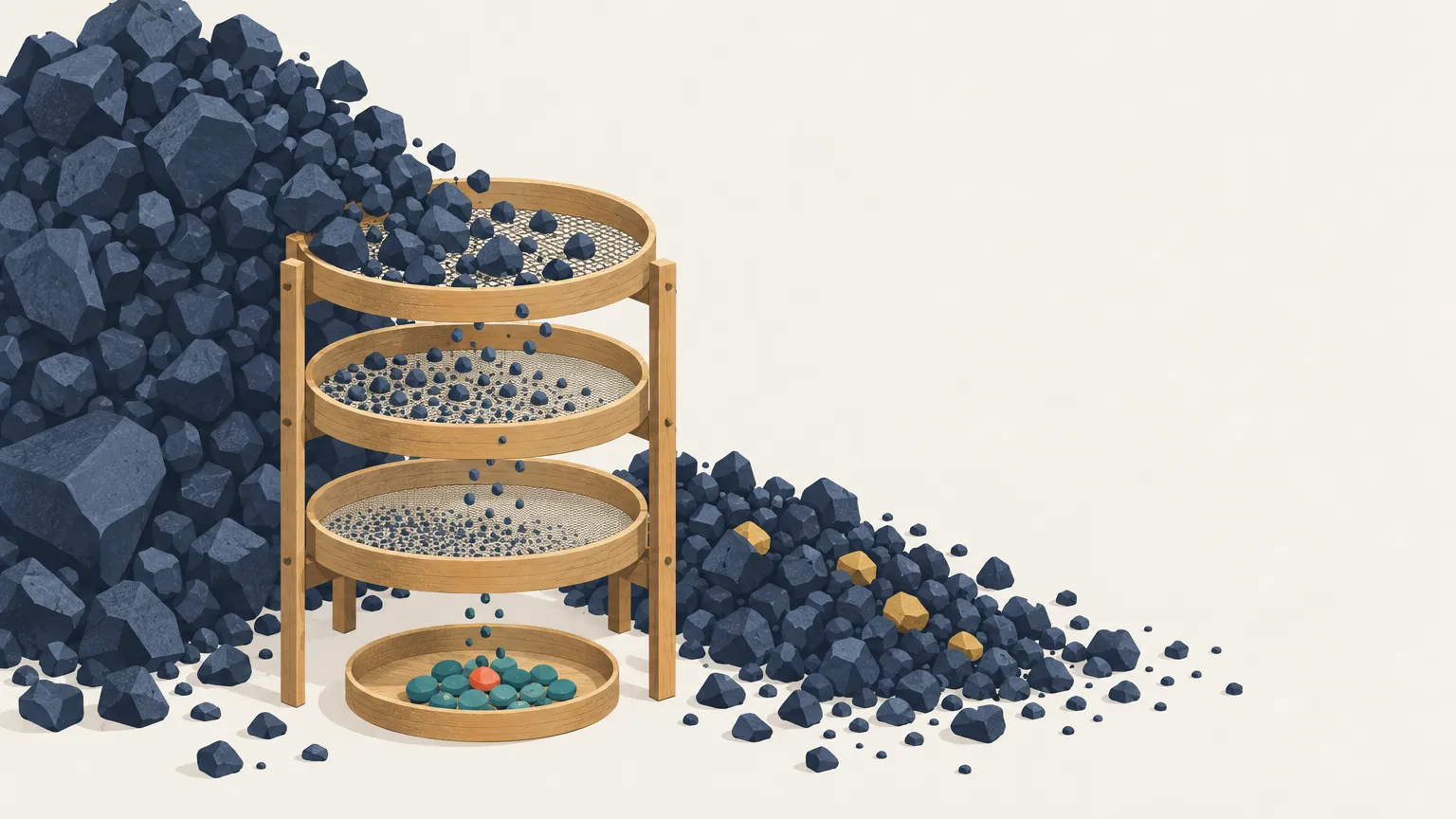
Aleph Alpha’s pipeline extracts more than 308B documents from Common Crawl, and after its rules and three kinds of deduplication 14.9B remain, 4.8% (computed). A quality ranking then cuts further. What survives supplies 3.82T of the 20T tokens Kolibri, its 78B-parameter model, draws in pre-training, counting repeats. Rephrased text seeded from the same crawl adds more, as do other web datasets.
Each lab building on web text has to decide what to throw away, by what test, and whether “throw away” should mean delete or only make rarer. Reports give plenty of one kind of number, the share a step removes, and little of another, what removing it did to the finished model. Aleph Alpha reports no ablation (an experiment that removes one piece) of its own for any rule or deduplication step. So this article keeps two questions apart: how much a step removes, and what we know it buys.
Why running out matters
A budget is the number of tokens a run will read, counting repeats. If a filter keeps a share of a pool of tokens, a budget repeats the survivors about times. On a small budget a strict filter causes no repeats. On a large one the same filter forces them, and a model learns less from a repeated document than from a new one. On subsets of a web corpus called C4, in runs up to 178B tokens, Muennighoff et al. find that up to four epochs cost “negligible” loss compared with unique data. With compute extended by their fitted law, gains continue to around 16 epochs, and by 40 further repeating is worthless. Loosening the filter avoids repeats and lowers the average. The choices in this article all sit on that line.
A filter keeping 25%: 4.0 repeats on a budget of 100% of the pool, 0.2 on a budget of 5%.
What goes in, and who says what
Common Crawl is a public archive of the web, published as a series of crawls called snapshots. A page can turn up in many of them, so a raw count of documents is partly a count of copies. Four of the 16 labs whose models this site tracks name it as a source (Aleph Alpha, NVIDIA, Poolside, and DeepSeek for its multimodal crawl). Others say “web”, which may or may not mean the same thing.
Filtering isn’t in modeling code, so we read technical reports first, then cards and official blogs. A blank below means we searched and found nothing, and doesn’t mean a lab skipped the step. Kolibri’s report is the most detailed public account, so it’s our worked example, and we don’t call it typical.
Besides lab reports we lean on public curation studies, which built web datasets and tested them on small models: DataComp-LM (DCLM), RefinedWeb, FineWeb and its successor FineWeb2, Dolma 3 (the dataset of the Olmo 3 model), and NVIDIA’s Nemotron-CC. Those are papers and datasets outside this site’s map, apart from NVIDIA’s link to its own.
As in the primer, a proxy is a small model trained to stand in for a run nobody can repeat. “A 7B proxy at 138B tokens” means 7 billion parameters reading 138 billion tokens. Scores come in a few kinds. MMLU is a four-way multiple-choice knowledge test, where chance is 25%. CORE is DCLM’s average over 22 tasks, rescaled so that chance is 0 and perfect is 100 (Fang et al. print it from 0 to 1). HumanEval is a small coding test, and pass@1 the share of problems whose first solution passes.
One funnel
Kolibri’s rules run in two parts: nine steps on everything, then a separate branch for each kept language. Of the 253.4B removed (82%), 171.5B go in the first part and 81.9B in the branches. That isn’t 82% junk, as the rest of this section shows.
The first filter comes before any of this. An extractor turns raw HTML into text, and Kolibri uses Resiliparse. In Nemotron-CC, swapping one extractor for another gained 28.6% more high-quality tokens on 13 snapshots, and on DCLM’s 1B proxy extraction moved CORE by as much as 3.8 points. Kolibri’s funnel starts after extraction, and apart from that NVIDIA paper no lab in our map reports what its extractor loses.
The hatched segment can’t be read as language selection either, though that’s plausible. Language identification (fastText, a small and fast linear text classifier, on the first 5,000 bytes) is the last of the nine steps, after rules on length, symbols, list lines and a block list of domains. The report gives no split. Two comparisons show that either could dominate: run early in DCLM, an English filter takes 50.8% of documents, and in Dolma 3, whose rules Kolibri’s extend, length and symbol rules take 62.5% of the pool.
A step’s share depends on what ran before it. Dolma 3 runs its English filter near the end and it takes 2.44% of the pool. Its authors call those rules commutative and put language late because it’s slow. That holds for rules that only drop documents, where order changes each step’s share and not the result. It fails for a step that edits text: removing lines can push a document under a length limit it passed before. Order across stages also differs. Nemotron-CC deduplicates before it classifies, FineWeb2 before it filters, and Kolibri does the reverse. We found no paper that tests the difference.
Every bar counts documents, and no stage has a published token count. A rule against pages under 50 words removes many documents and few tokens, so the token loss is probably smaller than 82%, by an amount nobody prints.
Inside the branches, the repetition rule, which drops documents that repeat their own lines or n-grams too much, removes the most at that position: it keeps 68.4% of English documents and 66.5% of German (we call the share a step keeps its yield). The mean-word-length range, the report’s example of German tuning, keeps 99.98%. Yields can’t rank value, and no quality classifier is in this funnel: its ranking comes afterward and cuts by tokens.
Rules
The cheapest test is a rule, which needs no model or labels. Kolibri’s drop a document with fewer than 50 or more than 100,000 words, or more than 0.1 hash or ellipsis symbols per word, or, in English, with more than 30% duplicate lines. Among the 16 labs, four state such rules for text (Aleph Alpha, NVIDIA, Moonshot, and Poolside on M.1), and only Aleph Alpha publishes thresholds.
These rules are inherited. Kolibri’s extend Dolma 3’s, which descend through DCLM and RefinedWeb from the appendix of DeepMind’s Gopher paper (Rae et al., 2021), with several of the same numbers. The German settings follow FineWeb2. Kolibri’s card says statistics were kept for “tuning heuristics appropriately”, and the report publishes no experiment behind any threshold. The one rule choice it backs with ablations is someone else’s: two rules from the MADLAD-400 filter, following Dolma 3, a step that drops a further 13.9B English documents.
Rules also discard good documents. Poolside on its first Laguna model, M.1: “broader rules removed more noise at the cost of discarding useful mid-quality documents, while highly precise rules covered only a small fraction of the noisy tail”. Nemotron-CC’s filters remove 18.1% of the tokens one classifier rates as high quality, so it applies them only to low-quality data. On an 8B proxy at 1T tokens, with no seed count given, that arm scores MMLU 57.5 against 54.1 with filters everywhere and 55.5 with none, while the average of its other tasks barely moves (60.6, 60.9, 60.3). Its stated reason is token yield.
Rules are cheap against training: Olmo 3 prices its rule stage, language identification and classifier runs included, over 252.6B documents at about $11,300, and puts its 32B checkpoint at about $2.75M, at $2 per H100 hour.
Classifiers
A classifier scores a document against examples. DCLM’s fastText model learned to tell instruction-style text from a random sample of its rule-filtered pool, using about 400K documents. On a 7B proxy at 138B tokens, keeping its top 10% raised CORE from 38.3 to 41.0 and MMLU from 25.4 to 29.2 at one learning rate, and from 39.7 to 44.1 and 25.5 to 38.3 at a better one, so changing the learning rate changed the score about as much as adding the filter did. DCLM calls this “the most influential step in our dataset design”. The top 10% beat 15% and 20% there, at a budget small enough that repeats weren’t the problem.
The cost is that quality now means whatever the positive examples were. In one Nemotron-CC snapshot, only 10.1% of the documents rated high quality by the FineWeb-Edu or DCLM classifiers are chosen by both, about twice what unrelated classifiers would share at those rates (computed). FineWeb-Edu’s “heavily favors” education and history over business and travel, on purpose.
From rules to judges
An LLM can score a document on any question you can write as a prompt, and Aleph Alpha says it “could be wasteful to apply an LLM-as-a-judge to tens of billions of documents”. So it runs a judge on a sample and copies its opinion into something cheap. That’s knowledge distillation with hard labels.
Kolibri’s judge, Qwen3-32B, scores a fixed 1M-document English sample using more than 20 prompts, on educational value, chat-likeness and so on. Each scalar axis becomes a binary task, top quartile against bottom quartile, and the middle half goes unused. A small classifier learns each task and runs on the rest.
Those classifiers tell the judge’s top quartile from its bottom quartile on held-out documents with F1 0.945 and AUC 0.987 for a fine-tuned BERT, 0.913 and 0.971 for a small network on Luxical (a fast pretrained embedding), and F1 0.865 for fastText. That’s an easier task than ranking a crawl. If the two classes are balanced and F1 is on the top class, a classifier that always says “top” already gets 0.667, and Kolibri’s English line, 40% of token mass up a blend of scores, probably falls in the middle half nobody trained on. Aleph Alpha prints no cost for any of this. For scale, FineWeb-Edu’s classifier took 6,000 H100 hours over 15T tokens.
Five scores then get combined. Weights are chosen by training 0.4B proxies on the top 25% of tokens under 26 sampled weightings, recording mean bits per byte on benchmark text, and fitting a Gaussian-process surrogate, a smooth model of score against weights. Bits per byte (BPB) is cross-entropy loss in bits per byte of text. It’s a proper scoring rule, so a gap between two models on one text is a real difference in how close their predictions are to it. Kolibri’s report doesn’t say which text. Olmo 3, in the same family of pipelines, scores only the gold answer or solution as a continuation of the prompt, divided by the answer’s bytes. That rewards predicting the wording of the right answer, which is a different test from picking the right option.
Dot: mean. Bar: 95% credible interval. n: seeds. Each panel has its own axis, and neither starts at 0.
Kolibri’s Table 10 is the one measured effect of a quality score we found in a report on a model in our map. On a mixture-of-experts proxy (7.8B parameters, 0.6B active per token), optimised annotations reach 0.618 against 0.868 for fastText’s top 25%. Five caveats go with it.
- The weights were chosen on BPB over these same benchmarks, so neither scale is a held-out test. fastText alone was one of the 26 weightings, one of the scores is a head for MMLU usefulness, and MMLU is among the benchmarks.
- The gap isn’t uniform. On the QA subset the two arms overlap (0.830±0.036 and 0.887±0.025). If the report’s means are unweighted, the other five benchmarks, mostly code and math, score 0.533 against 0.860 (computed). So the gap may reflect which domains each selection keeps as much as what either calls quality.
- The report puts the probability that this mix beats fastText at 0.93, on an “overall” figure it doesn’t print for fastText. With the printed English intervals, a Student-t posterior for each arm gives about 0.999 for a gap of 0.25 (computed). The same model gives 0.987 for the report’s 0.98 against Origin, and 0.93 would need a gap near 0.01, so we can’t reconcile them. fastText here has two seeds.
- The 0.4B values are odd in themselves: 3.8 to 4.7, against 0.62 to 0.88 on the MoE proxy and about 0.7 to 1.1 for Olmo 3’s 1B proxies at 100B tokens, which may not use the same text. Kolibri’s 30M swarm also predicts about 3.67, on a wider set of benchmarks. The report doesn’t comment, so we can’t say whether that’s the model or the column, and this is the run that chose the weights.
- These proxies draw a few percent of the selected pool (our estimate from 14.9B documents at DCLM’s 883 tokens each; the report gives no pool size), so few documents repeat. Such a run measures what selection does to the mix and not what it costs in repetition, so stricter cuts look better than they would on a full budget.
The report tests no score on Kolibri itself.
Other labs give less. Poolside tags documents with Propella, an open annotation model from other authors, with no formula for its composite score. Z.ai scores math and science candidates with language models and keeps the “most educational content”, and elsewhere uses a classifier to recover “otherwise medium-low-quality data”. A judge also isn’t guaranteed to do better: on DCLM’s 1B proxy, one LLM prompt reached CORE 28.6, against 30.2 for fastText.
Cut or rank
Once every document has a score, you can delete below a line or sample by score, and labs differ on which.
Poolside makes the argument. Its two Laguna models, M.1 and then XS.2, were both “trained on more than 30T tokens”, from a pool of about 27T unique tokens, so the change between them wasn’t budget. M.1 used a high-precision pipeline, which “exposed two bottlenecks: (1) excessive repetition in high-value subsets and (2) suboptimal allocation of data budget across different sources”. Poolside concludes that strategies “aggressively removing noisy documents to improve average quality … are not optimal for larger token budgets”, with no threshold for “larger”. Kolibri’s budget is 20T from a pool of 29.3T materialised tokens, so the two aren’t clearly on opposite sides of any line, and tokens from different tokenisers aren’t the same size.
For XS.2, after parsing, language identification and deduplication, a composite score rejects 25.8% of web samples outright, “recovering roughly 34% of high-quality documents previously excluded” by earlier rules. Survivors go into eight buckets by score, and each bucket is drawn at a set rate: one in the 0.006x bucket is drawn about 170 times less often than one at 1x.
Effective share phi = 0.195 (computed)
Kolibri English: lowest two of five tiers deleted, weights within the rest not published; phi at most about 0.6
Sampling by weight draws from the retained documents in proportion to , and nothing corrects for it afterwards, so the weights define what the model trains on. A cut is the case where is 0 or 1. One number measures how narrow any such curve is, the effective share of the pool (Kish’s effective sample size):
A cut keeping 30% has . Poolside’s weights give (computed), about the concentration of sampling evenly from the top fifth of retained documents, on this measure (the actual top fifth gets 83% of draws). If training draws documents per retained document, the document behind a typical draw goes in at a rate of about , five times . Poolside prints no , so the count itself is unknown. Once reaches 1, that’s about five times the repeats of even sampling on the same budget. Below 1, even sampling needn’t repeat at all, while this curve still repeats its top buckets. Kolibri’s English cut keeps about 60% of token mass, and weighting within it can only lower that. Units and stages differ, so this isn’t a precise comparison, but ranking isn’t automatically the gentler choice. The gain from ranking is reach: every retained document has some chance, and the lowest four buckets still get 4.7% of draws.
Aleph Alpha cuts by tier. Documents are ranked and split into five tiers of equal token mass, and it drops the lowest two in English and the lowest one in German. The roughly 60% and 80% it keeps follow from the equal masses, and the report gives no ablation for where to cut. Kept tiers enter its mix as separate sources (the next article).
NVIDIA’s reference pipeline, Nemotron-CC, argues that the roughly 90% DCLM and FineWeb-Edu remove “may not be the most effective strategy when training larger models over longer token horizons”. Its dataset includes low-quality text rephrased by an LLM. Yet its 8B reference run at 15T uses medium, medium-high and high tiers, and Nemotron 3 Ultra’s printed mix has no low tier either. It also uses synthetic crawl text labelled medium and high, 33% of its first phase (computed); the report doesn’t say how that’s made, and Nemotron-CC’s is rephrased. A companion paper, Feng et al., finds on an 8B model that “eliminating the tail-end of the web crawl data” helps. So labs facing one scarcity pull three levers: deleting, reweighting and manufacturing unique text (the synthetic data article).
We found no controlled comparison on a final or full-budget model, and the nearest results are proxies.
- Olmo 3 shrinks the pool with the budget so that repetition matches a 4.51T run, on a 1B model at 100B tokens. That’s the fix for the proxy problem above. Its quality-aware upsampling beats the best flat cut in each column on BPB, by little on QA (1.000 against 1.031) and more on math (0.740 against 0.843) and code (0.719 against 0.880), with no seeds shown. Its example curve also discards the bottom 40%, so it’s a hybrid.
- Fang et al. find that a strict filter repeated for ten epochs can beat its ten-times-larger superset at 12.6B parameters and 252B tokens, with weight decay retuned, while trailing one epoch of fresh strict data (CORE 0.523 against 0.550, no error bars, and the superset’s score appears only in a plot). They expect this is “likely” to fail once data is much more constrained than compute.
- Mohri et al. find that with enough compute the unfiltered pool has the lowest loss, with benchmark results in an appendix that are much noisier and show “roughly the same” trends, on dense models with no data weighting and pools of at most 10B tokens. They extrapolate the crossing for a 240T pool to near FLOPs, against about for DCLM’s largest benchmark scale.
Poolside’s claim rests on cited work, on M.1, whose repetition factor it doesn’t print, and on “targeted smaller scale experiments” it doesn’t describe. It reports no filter-only result, and it changed the filter together with synthetic rephrasing, the mix and the model size, which is much smaller for XS.2.
Deduplication: three tests for “the same”
Aleph Alpha’s stages remove 39.9B of the 54.8B documents that reach them, 73% (computed). That doesn’t say how redundant the web is. Most of it is exact copies among the many pooled crawls, and the share rises with the pool: in one DCLM test of its Bloom filter, tokens removed went from 29% to 46% as the pool grew fivefold.
Exact copies
Hash each document’s bytes and keep one per hash. Aleph Alpha uses a 128-bit xxHash on unnormalised text, first within each snapshot and then across all of them, keeping the earliest copy. The pass across snapshots removes 22.1B of 43.3B, the largest of the four steps after the rules. Each kept document records its copy counts, which “leave the decision how often to repeat a document to the mixing stage”. The report never says the mixer used them.
Near-duplicates
Two pages that differ by a date escape a hash. Cut each document into overlapping token 5-grams, called shingles, and measure two documents by Jaccard similarity : shared shingles over all distinct shingles. Comparing all pairs among Kolibri’s 21.16B documents would take about comparisons (computed), so nobody does.
MinHash (Broder, 1997) gives a cheap estimate. Apply a random hash function to every shingle of both documents. Across the two sets, the shingle with the smallest hash is equally likely to be any of them, and the two documents share that minimum exactly when it’s in both, so they agree with probability . Do this with many hash functions and each document gets a signature, a column of minima.
Locality-sensitive hashing then avoids the pairs. Split the signature into bands of rows, and hash each band into a table. Two documents meet only if a band lands in the same slot, so the work grows with documents and bands, never with pairs. A band matches with probability and all miss with probability , so:
Aleph Alpha uses 26 bands of 11 rows, 286 hashes per document, which gives 0.51 at and 0.99 at 0.85 (computed; the report states the same). Olmo 3 uses the same 26 by 11.
b = 26, r = 11, 286 hashes per document. P = 0.5 at s = 0.718. P at 0.80 = 0.903.
It then groups candidates into clusters and checks them on token 3-gram Jaccard at 0.80. Verification removes false candidates, which is why the signature can be small where RefinedWeb used 9,000 hashes, and it can’t recover a pair that never matched. In clusters that loss is smaller, since documents can meet through a third. In an idealised family of documents at pairwise 5-gram similarity 0.80, a document ends up alone about 10% of the time with one partner and under 0.1% with nine (simulated). Near the check’s own line the loss is larger: pages that pass 0.80 on 3-grams can sit near 0.70 on 5-grams, where a document stays alone about 60% of the time with one partner and about 10% with nine. So banding mostly loses small clusters. The report doesn’t say which document of a cluster survives.
Repeated substrings
The same 2KB menu on a million otherwise different pages escapes both tests. A suffix array lists every position in the text sorted by what follows it, so repeated runs sit next to each other (Lee et al., 2022). Within each of 41 three-snapshot English shards (groups of snapshots processed together), and 7 German ones, Aleph Alpha keeps one occurrence of any repeated run of at least 500 bytes and cuts the others. That removes only 0.8B documents and 21.3% of the bytes reaching it. The stated price: “The cuts join the text on either side without a check for coherence, and cut documents skip the heuristic filters.”
Minimum length matters. DCLM’s Bloom-filter deduplication (a compact hash-based test for “seen this before”) at 7B and 280B tokens scores MMLU 44.3 with a 13-gram minimum and 10 shards, and 32.5 with a 5-gram minimum and 32 shards, CORE nearly flat. At half that budget on 32 shards each, the gap is 28.7 against 26.3. The authors blame short repeated lines: “1 stick of butter” is a common 5-gram, and removing it from every recipe leaves broken text.
Semantic duplicates
Embedding similarity catches paraphrases. Liquid calls it the “largest reduction” in its SFT pipeline, with no number, and DCLM’s one measured arm, at 1B, scores 27.1 CORE against a 27.5 baseline.
What deduplication buys
We found no controlled test at 10T or more, and no lab in our map gives a benchmark number for a deduplication step. Smaller studies disagree, largely according to what they measured.
Memorization has the clearest result. On a 1.5B model, Lee et al. find the share of generated tokens copied from training falls from 1.926% to 0.138% after one epoch, with perplexity no worse. Benchmarks gain a little on small models: RefinedWeb’s stage adds 0.2 to 2.9 points on four other datasets, and DCLM’s methods add 0.9 to 2.1 CORE at 1B when used singly, with some gaps inside variance. Muennighoff et al. find “deduplication does not help” downstream on C4, where deduplicated data repeats four times to fill an 84B budget.
Fang et al. show that what follows deduplication matters. On an already filtered dataset (7B, 138B tokens), uniform sampling beats global deduplication then sampling (CORE 44.4 against 41.7, MMLU 42.2 against 28.5), because uniform sampling favours documents with many copies. Keeping one copy each and ranking by classifier score and copy count together beats both (46.1, 46.0).
FineWeb (1.71B parameters, 350B tokens) is the nearest test of scope. Global fuzzy deduplication, removing up to 90% of old snapshots, showed “little improvement” over none, while per-snapshot deduplication matched RefinedWeb. The authors’ hypothesis is that removing giant clusters helps and removing small ones “can harm performance”, because what survives is unique and often worse. Three things limit this. FineWeb sampled what was left at random, and pipelines that rank afterwards may not pay the price. Its authors moved to global deduplication in FineWeb2, reweighting by cluster size. And its own simulation warns that small runs can barely see the effect, since at 1B tokens drawn from a 20T set almost every document is unique anyway.
template clustergood page, recrawledone-off, low quality
Toy: 42 good, 64 one-off and 8 template documents survive.
Labs choose different scopes. Poolside: “Snapshot-level fuzzy deduplication is preferred because it gives higher performance on knowledge benchmarks. Indeed, we observed that similar web pages across snapshots are statistically more likely to contain relevant facts.” It gives no numbers, baseline or method. Aleph Alpha removes byte-identical copies across every snapshot, and runs fuzzy deduplication in 30 English and 6 German shards, dealing snapshots out in turn, “so near-duplicates in different shards remain”. Olmo 3 deduplicates exactly across the whole pool, accepting that this “necessarily discards the quality signal from duplicate counts”, and adds repetition back by quality score, the curve above. Neither Poolside nor Aleph Alpha publishes a comparison with the other’s choice.
Shards aren’t only a stance. DCLM calls them a trade of scalability against yield, and one of its tests projects 3.9T tokens at 32 shards and 1.3T at one, with CORE about a point apart. Kolibri’s deduplication also stops at the crawl: Aleph Alpha reports cross-dataset deduplication for mid-training only, so as far as it reports, a page in both the crawl and another pre-training dataset stays in both, and its per-dataset cap on repeats counts each copy separately. No report measures this.
Aleph Alpha says the copy count “correlates with document quality”, citing Fang et al., whose curve of fuzzy copies against classifier score is small, non-monotone and measured on filtered data. FineWeb2 finds a U shape, and Lee et al. find templates, bot replies and licences among the most repeated text. We read that as some signal at moderate counts and boilerplate at the top, across results that don’t share a method.
Benchmark decontamination
A test question in the training data turns a benchmark into a memory test. Decontamination finds and removes such text, and its scope is the main fact. Of the 16 labs, four describe it. Google gives one sentence under pre-training (“We filter data to decontaminate benchmarks”). Aleph Alpha treats its mid-training and SFT pools. NVIDIA treats post-training data and one mid-training stage. Liquid treats SFT data.
Aleph Alpha cites Bordt et al. for the logic: contamination early in training is forgotten, and near the end it isn’t, so it decontaminates the late pool. It indexes 5-grams of questions and 3-grams of answers from its 226 evaluation tasks, weights each by rarity, and drops whole documents with AI2’s decon tool: 1.5M of 8.3B, 0.018% of documents and 0.06% of tokens. “The pre-training pool remains potentially contaminated.” Most of what it finds isn’t web text: synthetic instruction data accounts for 67% of removals, and web crawl text for 9%, at 0.006% of its documents.
Aleph Alpha reports two proxy results, with arm sizes unstated, and one from Kolibri itself. With removed documents left at their usual tiny share, runs with and without decontamination “track each other within noise”, so “the contamination is not measurable” at that scale. The report doesn’t read that as safety: the contaminated share is about the same at any scale, but the number of times a document is seen grows with the budget. As an upper bound, adding every removed document back, at 8.2% of the proxy mix’s tokens, “inflates HumanEval by 42 points, MMLU by 29 and TriviaQA by 28” and halves BPB on benchmark text.
On Kolibri itself, a completion counts as recited if it nearly equals the benchmark’s reference solution. During pre-training, 22% to 95% of HumanEval completions are recited, and pass@1 follows that share, with a correlation of 0.90 over 96 evaluations. Part of that is arithmetic, since a recited solution passes. The lab concludes that those scores aren’t comparable with a decontaminated model’s, and plans to decontaminate that pool next time.
Mid-training on the decontaminated mix then cuts recitation below 10% within 0.3T tokens, and English pass@1 falls from 80.0 to 70.0. By the end of mid-training recitation is back to 48% in English and 47% in German. New exposure can’t explain that if the pool is clean. The report calls it “a checkpoint-level state”, and it also says the method misses “reference solutions that appear without their prompt”. So a low recited share at one checkpoint doesn’t show forgetting, and the lab also reports its aggregate without HumanEval.
Kolibri’s run can’t test Bordt’s result in either direction. Bordt’s finding is that questions inserted up to 144 times can be forgotten once clean data passes five times Chinchilla, the compute-optimal budget of about 20 tokens per parameter, on models up to 1.6B parameters and 40B tokens, with continued training of OLMo-7B in support. Kolibri’s 3.44T of mid-training is under that line counted on total parameters (7.8T) and over it counted on active ones (0.35T), Bordt’s models are dense, and Kolibri’s exposure count isn’t published. Bordt also finds overfitting strongest for examples seen throughout training, which fits what Kolibri sees in pre-training.
Detection has limits of its own. NVIDIA checks post-training data against 30 benchmarks with n-grams and embeddings, then asks an LLM judge (Claude Opus 4.6) to label each candidate, removing 20,671 samples, around 0.09%. That rate and Aleph Alpha’s 0.06% of tokens differ in unit, pool and stage. Its judge caught 87.5% and 79.1% of planted variants of Terminal-Bench 2.1 and GPQA Diamond, with one false positive among 12,763 negatives, which are questions from other benchmarks. “Ground-truth contamination labels do not exist for real data”, so neither recall nor precision on real data is known.
PII, safety, licence, provenance
Reports say least about these steps. Three labs state that they remove personal data (PII) from pre-training text. Aleph Alpha detects categories by regular expression with a validator and drops a document “whose redacted bytes exceed 15 % of its length”, and its card reports an ablation on a 750M-row sample with “no clear performance difference in either direction”, model and metric unstated. Google and DeepSeek name no method.
Three labs state safety filtering on pre-training data. OpenAI reuses “the CBRN pre-training filters from GPT-4o” (chemical, biological, radiological, nuclear). Google filters child sexual abuse material “at multiple stages”. Aleph Alpha uses a URL list and, for English web text, keywords, and states the gap: “no dedicated CSAM detection was applied”. Thinking Machines says its steps “may include deduplication and filtering”, and the hedge is theirs.
NVIDIA removes source code without a permissive licence. Aleph Alpha alone describes screening third-party datasets: it checks whether whoever crawled the data honoured opt-outs such as robots.txt, and if not, “we exclude such datasets from our training”. It gives no count, and the section doesn’t discuss Common Crawl itself. “Opt-out” and “robots” occur in no other lab’s primary documents in our corpus.
The steps compared
| Step | Labs of 16 | Who | What has been measured | Main caveat |
|---|---|---|---|---|
| Quality classifier or score | 6 | Aleph Alpha, NVIDIA, Poolside, Moonshot, Z.ai, DeepSeek | Kolibri Table 10, proxies, BPB; DCLM, 7B | DeepSeek multimodal; NVIDIA by reference |
| Rules | 4, and 2 scoped | Aleph Alpha, NVIDIA, Moonshot, Poolside; DeepSeek (multimodal), Z.ai (long-context length) | Yields at labs; Nemotron-CC, 8B | Only Aleph Alpha gives thresholds |
| LLM-scored documents | 3 to 4 | Aleph Alpha (distilled), Z.ai (direct), DeepSeek (multimodal), Poolside (Propella) | Table 10 | Poolside doesn’t call Propella an LLM |
| Language ID | 3 | Aleph Alpha, Poolside, NVIDIA (by reference) | None | NVIDIA’s 15 further languages: method unstated |
| Exact dedup, pre-training | 2 | Aleph Alpha, Moonshot (long context) | Small proxies only | Liquid on SFT |
| Fuzzy dedup, pre-training | 5 | Aleph Alpha, NVIDIA (by reference), Poolside, Z.ai (code), Moonshot (long context) | Poolside direction only; FineWeb, 1.71B | Method named only by Aleph Alpha |
| Substring dedup | 2 | Aleph Alpha, NVIDIA (by reference) | DCLM, 1B and 7B | |
| Decontamination | 4 | Google, Aleph Alpha, NVIDIA, Liquid | Kolibri proxies, upper bound | Only Google under pre-training |
| PII | 3 | Aleph Alpha, Google, DeepSeek | Kolibri card: no clear difference | Metric unstated |
| Safety | 3 | OpenAI, Google, Aleph Alpha | None | Thinking Machines hedged |
| Licence | 2 | NVIDIA (per file), Aleph Alpha (per dataset) | None | Different levels |
Filters against synthetic and templated text appear at three labs (DeepSeek on web text, Z.ai on math and science, Aleph Alpha on its long-context mix), and audits or human screening at four (Aleph Alpha, Liquid, NVIDIA, Moonshot), on post-training or synthetic data.
Where the models in the map sit
For text, unless noted.
| Lab | Sources stated | Filters on base-model data | Dedup on base-model data |
|---|---|---|---|
| Aleph Alpha | Own Common Crawl pipeline, 78 datasets | Rules with thresholds, language ID, distilled judge, tiers, PII, URL and keyword lists | Exact, MinHash, substring |
| Poolside | Common Crawl, code, academic, synthetic | Language ID, composite score, 25.8% rejected, then ranked | Snapshot-level fuzzy |
| NVIDIA | Common Crawl, GitHub, FinePDFs, others | By reference to Nemotron-CC; rules only for 15 languages; tiers; permissive licences on code | By reference |
| Moonshot | Web, code, math, knowledge | Rules, classifier, per domain | “deduplication”; exact and fuzzy in long context |
| Z.ai | Web, code hosts, books, papers | Classifiers; LLM scoring and anti-synthetic in math and science | “fuzzily deduplicated” (code); “deduplication” (long context) |
| DeepSeek | Web, Common Crawl for multimodal, licensed data | Anti-template, anti-auto-generated; PII; quality models for multimodal | Multimodal; overlap with text-only samples replaced |
| Xiaomi | Web, books, papers, code | “multi-dimensional data filtering” (MiMo-7B) | |
| Web, code, images, audio | Quality, PII, CSAM, decontamination, no method | ||
| OpenAI | “text-only dataset” | CBRN | |
| Thinking Machines | Internet, repositories, third parties, synthetic | “may include” | “may include” |
| Mistral | Web, code, documents | “higher-quality” data, test unstated | |
| Tencent | “fine-grained data cleaning”, stage unstated | ||
| Liquid | Mix shares only | SFT only | SFT only |
| MiniMax | Interleaved data | ||
| Qwen | Modality token counts for Omni | ||
| StepFun |
Easy to get wrong
- “82% of the crawl is junk.” The first bar counts copies and other languages along with junk, and counts documents, not tokens.
- “Soft means gentle.” Poolside’s curve has a smaller effective share than Kolibri’s cut. Under ranking the tail stays reachable, which says nothing about how narrow the sampling is.
- “Kolibri uses copy counts as a quality signal.” It records them and leaves the choice to the mixer, and never reports using them.
- “NVIDIA’s large models train on rephrased low-quality text.” The Nemotron-CC dataset contains some, but its 15T run used medium tiers and up, and Ultra’s mix has no low tier.
- “F1 0.913 means the classifier nearly reproduces the judge.” That’s on the extremes, with the middle half left out.
- “Four epochs is the limit of repetition.” That’s as far as the loss difference stayed negligible on C4 at small scale.
- “The judge recovers 87.5% of contamination.” That’s its recall on planted variants of one benchmark. The rate on real data is unknown.
Check yourself
- Kolibri’s fuzzy step uses 26 bands of 11 rows. Two documents have similarity 0.60 on 5-grams. What’s the chance they become a candidate pair? And with 14 bands of 8 rows?
Answer
. With FineWeb’s 14 by 8, . Fewer rows per band make a match easier, so the curve starts earlier and more pairs go on to verification. - A report says a filter removes 40% of documents. Another says its filter removes 3%. What can you conclude about which matters more?
Answer
Nothing. A step’s share depends on what ran before it and on the unit, and neither number says what removing those documents did to a model. - Poolside rejects 25.8% of web samples and Kolibri’s funnel removes 95% of documents. Why can’t you call Poolside 3.7 times gentler?
Answer
Poolside’s 25.8% comes after parsing, language identification and deduplication. Kolibri’s 95% starts from raw extraction. The nearer comparison is its tier cut, about 40% of English tokens, in a different unit. And Poolside’s sampling then has an effective share of 0.195. - A curve has weights 0 on half of a pool and 1 on the other half. What’s ? If you draw as many documents as the pool holds, at what rate does each kept document go in?
Answer
and , so , the kept share. With , that’s per kept document. - Why doesn’t the 42-point HumanEval inflation show that contamination inflated Kolibri by 42 points?
Answer
It’s an upper bound on a proxy, with removed documents added back at 8.2% of the mix, where the pool’s rate is 0.06% of tokens. With natural rates, the same report measures nothing at proxy scale. Its evidence about Kolibri itself is the recitation data.
In the map
Methods
- Common Crawl 1 source
- Heuristic filtering 4 sources
- Heuristic web-document filtering and cleanup 1 source
- Language-specific fastText routing and filtering 1 source
- Distilling LLM-judge annotation axes into binary classifiers 1 source
- Multi-dimensional document quality scoring 1 source
- Propella multi-property document annotation 1 source
- Conservative model-based noise filtering 1 source
- Ranking retained documents by continuous contribution score 1 source
- Equal-token-mass language-specific quality tiers 1 source
- Filtering batched auto-generated and templated web content 2 sources
- Nemotron-CC pipeline 1 source
- Exact text deduplication 2 sources
- MinHash locality-sensitive hashing fuzzy deduplication 1 source
- Substring deduplication 1 source
- Snapshot-level fuzzy deduplication 1 source
- Semantic deduplication 1 source
- Benchmark decontamination 4 sources
- Benchmark decontamination by n-gram and semantic matching 1 source
- Personally identifiable information redaction 2 sources
- CBRN safety filtering of pre-training data 2 sources
- CSAM filtering 3 sources
- Permissive-license filtering 2 sources
- Third-party data-source compliance screening 1 source
Taxonomy nodes
- data curation 11 methods
- data sourcing 37 methods
- data filtering 145 methods
- deduplication 15 methods
Further reading
- Kolibri report, §2.3 and Appendix D: https://aleph-alpha.com/downloads/tech-report.pdf. All thresholds, both funnel figures, decontamination in full.
- Laguna report, §3.2: https://poolside.ai/assets/laguna/laguna-m1-xs2-technical-report.pdf. The argument for high recall at large budgets.
- Nemotron 3.5 report, §3.12 and Appendix C: https://research.nvidia.com/labs/nemotron/files/NVIDIA-Nemotron-3.5-Super-and-Lightning-Technical-Report.pdf. Decontamination with an LLM judge and a planted test.
- Su et al., Nemotron-CC, arXiv:2412.02595, and Feng et al., Two-Phase Pretraining, arXiv:2412.15285. Tiers, rephrasing, and a test of dropping the tail.
- Li et al., DataComp-LM, arXiv:2406.11794. A large public ablation of a curation pipeline.
- Penedo et al., FineWeb, arXiv:2406.17557, and FineWeb2, arXiv:2506.20920. Why global deduplication disappointed, why small runs can’t see it, and a change of course.
- Lee et al., Deduplicating Training Data Makes Language Models Better, arXiv:2107.06499. The two tools still in use, and the memorization result.
- Fang et al., Datasets, Documents, and Repetitions, arXiv:2503.07879. Repeats, weight decay and document counts set on purpose.
- Muennighoff et al., Scaling Data-Constrained Language Models, arXiv:2305.16264. What “four epochs” means.
- Bordt et al., How Much Can We Forget about Data Contamination?, arXiv:2410.03249. When contamination fades, and its limits.
- Olmo 3, arXiv:2512.13961, §3.4 and Table 39. A pipeline in the same family, with quality-aware upsampling.
- Mohri et al., A Bitter Lesson for Data Filtering, arXiv:2605.19407. The case that no filter wins given enough compute.
- Broder, On the resemblance and containment of documents, 1997, and Leskovec, Rajaraman and Ullman, Mining of Massive Datasets, ch. 3. MinHash and banding.
- Rae et al., Gopher, arXiv:2112.11446, Appendix A. Where the rules’ numbers started.